Computational Fluid Dynamics group
@CFDonia • 3,875 subscribers
Fluid Dynamics, Environmental Flows, Weather & Climate, Turbulence, Scientific Computing @UConn. We love art and computer programming (led by G. Matheou)
Shorts
![Kinetic energy dissipation rate in two-dimensional turbulence. Logarithmic contours. Plots with Matplotlib Data available here: #Python script to generate plots: import numpy as np import matplotlib as mpl import matplotlib.colors as colors import matplotlib.pyplot as plt from netCDF4 import Dataset f1=Dataset(' mode='r') dissipation = f1.variables['dissipation'][:,:,:] x = f1.variables['x'][:] y = f1.variables['y'][:] n = dissipation.shape for k in range(0, n[0]): fig, ax = plt.subplots(1,1, figsize=(8,8)) cs1 = ax.contourf(x, y, dissipation[k,:,:], np.logspace(-5,1,101), cmap='Blues_r', extend='both', norm=colors.LogNorm()) ax.set_aspect('equal') ax.xaxis.set_ticks(range(0,7)) ax.yaxis.set_ticks(range(0,7)) ax.set_xlabel(r'$x$') ax.set_ylabel(r'$y$') fname = 'frame.' + str(k) + '.png' plt.savefig(fname, dpi=200, pad_inches = 0.1) print(fname) plt.close()](https://image.24vids.com/tw-1657043268364902403/ext_tw_video_thumb/1657042233323843587/pu/img/4dddFVajks_nWEw1.jpg)
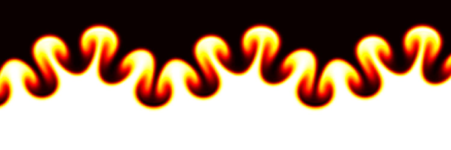
Kinetic energy dissipation rate in two-dimensional turbulence. Logarithmic contours. Plots with Matplotlib Data available here: #Python script to generate plots: import numpy as np import matplotlib as mpl import matplotlib.colors as colors import matplotlib.pyplot as plt from netCDF4 import Dataset f1=Dataset(' mode='r') dissipation = f1.variables['dissipation'][:,:,:] x = f1.variables['x'][:] y = f1.variables['y'][:] n = dissipation.shape for k in range(0, n[0]): fig, ax = plt.subplots(1,1, figsize=(8,8)) cs1 = ax.contourf(x, y, dissipation[k,:,:], np.logspace(-5,1,101), cmap='Blues_r', extend='both', norm=colors.LogNorm()) ax.set_aspect('equal') ax.xaxis.set_ticks(range(0,7)) ax.yaxis.set_ticks(range(0,7)) ax.set_xlabel(r'$x$') ax.set_ylabel(r'$y$') fname = 'frame.' + str(k) + '.png' plt.savefig(fname, dpi=200, pad_inches = 0.1) print(fname) plt.close()
385,238 次观看
![Following many two-dimensional turbulence animations, it is time to share computer code! Implementation of a vorticity-streamfunction method with a pseudo-spectral discretization + third-order Runge-Kutta for time integration (our CFD class semester project). The MATLAB code: M = 256; % number of points N = M; Lx = 2*pi; Ly = 2*pi; nu = 5e-4; % kinematic viscosity Sc = 0.7; % Schmidt number beta = 0; % meridional gradient of Coriolis parameter ar = 0.02; %random number amplitude b = 1; % mean scalar gradient CFLmax = 0.8; tend = 200; % end time x=linspace(0,Lx,M+1); x(end)=[]; dx = Lx/M; kx=[0:M/2 -M/2+1:-1]*2*pi/Lx; y=linspace(0,Ly,N+1); y(end)=[]; ky=[0:N/2 -N/2+1:-1]*2*pi/Ly; dy = Ly/N; time = 0; index_kmax = ceil(M/3); kmax = kx(index_kmax); filter = ones(M,N); filter(index_kmax+1:2*index_kmax+3,index_kmax+1:2*index_kmax+3)=0; rng(64); [u, v, omega, psi, ddx, ddy, idel2, kk, k2]=deal(zeros(M,N)); for j=1:N ddx(:,j)=1i*kx; end for i=1:M ddy(i,:)=1i*ky; end for i=1:M for j=1:N idel2(i,j)=-kx(i)^2-ky(j)^2; end end idel2=1./idel2; idel2(1,1)=0; for i=1:M for j=1:N kk(i,j)=kx(i)^2+ky(j)^2; k2(i,j)=kx(i)^2+ky(j)^2; if kk(i,j) >= 6^2 && kk(i,j) <= 7^2 % forcing kk(i,j) = -kk(i,j); end if kk(i,j) <= 2^2 kk(i,j) = 8*kk(i,j); % large-scale dissipation end end end for i=1:M for j=1:N u(i,j) = cos(2*x(i))*sin(2*y(j))+ar*rand; v(i,j) = -sin(2*x(i))*cos(2*y(j))+ar*rand; end end uhat = fft2(u); vhat = fft2(v); omegahat = ddx.*vhat - ddy.*uhat; % make vorticity phi = rand(size(u)); phihat = fft2(phi); ncid = netcdf.create(' 'CLOBBER'); dimid_x = netcdf.defDim(ncid, 'x', M); dimid_y = netcdf.defDim(ncid, 'y', N); dimid_time = netcdf.defDim(ncid, 'time', netcdf.getConstant('NC_UNLIMITED')); varid_x = netcdf.defVar(ncid, 'x', 'NC_FLOAT', [dimid_x]); varid_y = netcdf.defVar(ncid, 'y', 'NC_FLOAT', [dimid_y]); varid_u = netcdf.defVar(ncid, 'u', 'NC_FLOAT', [dimid_x, dimid_y, dimid_time]); varid_v = netcdf.defVar(ncid, 'v', 'NC_FLOAT', [dimid_x, dimid_y, dimid_time]); varid_omega = netcdf.defVar(ncid, 'vorticity', 'NC_FLOAT', [dimid_x, dimid_y, dimid_time]); varid_phi = netcdf.defVar(ncid, 'scalar', 'NC_FLOAT', [dimid_x, dimid_y, dimid_time]); varid_dissipation = netcdf.defVar(ncid, 'dissipation', 'NC_FLOAT', [dimid_x, dimid_y, dimid_time]); varid_time = netcdf.defVar(ncid, 'time', 'NC_FLOAT', [dimid_time]); netcdf.endDef(ncid); netcdf.putVar(ncid, varid_time, 0, 1, time); netcdf.putVar(ncid, varid_x, 0, M, x); netcdf.putVar(ncid, varid_y, 0, N, y); netcdf.putVar(ncid, varid_phi, [0, 0, 0], [M, N, 1], phi); netcdf.putVar(ncid, varid_u, [0, 0, 0], [M, N, 1], u); netcdf.putVar(ncid, varid_v, [0, 0, 0], [M, N, 1], v); netcdf.putVar(ncid, varid_omega, [0, 0, 0], [M, N, 1], omega); netcdf.putVar(ncid, varid_dissipation, [0, 0, 0], [M, N, 1], 0*omega); dt = 0.5*min([dx dy]); nstep = 1; while time < tend psihat = -idel2.*omegahat; uhat = ddy.*psihat; vhat = -ddx.*psihat; u = real(ifft2(uhat)); v = real(ifft2(vhat)); omegadx = real(ifft2(ddx.*omegahat)); omegady = real(ifft2(ddy.*omegahat)); facto = exp(-nu*8/15*dt*kk); factp = exp(-nu/Sc*8/15*dt*k2); r0o = -fft2(u.*omegadx+v.*omegady)+beta*vhat; r0p = -fft2(u.*real(ifft2(ddx.*phihat))+v.*real(ifft2(ddy.*phihat)))+b*vhat; omegahat = facto.*(omegahat + dt*8/15*r0o); % update omega phihat = factp.*(phihat + dt*8/15*r0p); % update phi %%%% Substep 2 psihat = -idel2.*omegahat; uhat = ddy.*psihat; vhat = -ddx.*psihat; u = real(ifft2(uhat)); v = real(ifft2(vhat)); omegadx = real(ifft2(ddx.*omegahat)); omegady = real(ifft2(ddy.*omegahat)); r1o = -fft2(u.*omegadx+v.*omegady)+beta*vhat; r1p = -fft2(u.*real(ifft2(ddx.*phihat))+v.*real(ifft2(ddy.*phihat)))+b*vhat; omegahat = omegahat + dt*(-17/60*facto.*r0o + 5/12*r1o); phihat = phihat + dt*(-17/60*factp.*r0p + 5/12*r1p); facto = exp(-nu*(-17/60+5/12)*dt*kk); factp = exp(-nu/Sc*(-17/60+5/12)*dt*k2); omegahat = omegahat.*facto; phihat = phihat.*factp; %%%% Substep 3 psihat = -idel2.*omegahat; uhat = ddy.*psihat; vhat = -ddx.*psihat; % max(max(abs(real(ifft2(1i*ddx.*uhat+1i*ddy.*vhat))))) % divergence u = real(ifft2(uhat)); v = real(ifft2(vhat)); omegadx = real(ifft2(ddx.*omegahat)); omegady = real(ifft2(ddy.*omegahat)); r2o = -fft2(u.*omegadx+v.*omegady)+beta*vhat; r2p = -fft2(u.*real(ifft2(ddx.*phihat))+v.*real(ifft2(ddy.*phihat)))+b*vhat; omegahat = omegahat + dt*(-5/12*facto.*r1o + 3/4*r2o); phihat = phihat + dt*(-5/12*factp.*r1p + 3/4*r2p); facto = exp(-nu*(-5/12+3/4)*dt*kk); factp = exp(-nu/Sc*(-5/12+3/4)*dt*kk); omegahat = omegahat.*facto; phihat = phihat.*factp; phihat = filter.*phihat; omegahat = filter.*omegahat; time = time + dt; nstep = nstep + 1; CFL = max(max(abs(u)))/dx*dt+max(max(abs(v)))/dy*dt; if mod(nstep,20)==0 phi = real(ifft2(phihat)); omega = real(ifft2(omegahat)); dissipation = 2*nu*(real(ifft2(ddx.*uhat)).^2 + real(ifft2(ddy.*uhat)).^2 + real(ifft2(ddx.*vhat)).^2 + real(ifft2(ddy.*vhat)).^2); eta = (nu^3/mean(dissipation,'all'))^0.25; subplot(221); pcolor(x,y,omega'); title('Vorticity'); shading flat; axis equal tight; colorbar; drawnow subplot(222); pcolor(x,y,phi'); title('Scalar'); shading flat; axis equal tight; colorbar; drawnow subplot(223); pcolor(x,y,dissipation'); title('Dissipation'); shading flat; axis equal tight; colorbar; drawnow subplot(224); pcolor(x,y,u); title('u-velocity'); shading flat; axis equal tight; colorbar; drawnow fprintf(1,'step = %d time = %g dt = %g CFL = %g kmax*eta = %g %g\n', nstep, time, dt, CFL, eta.*kmax, eta.*kmax/sqrt(Sc)); [~, dim_time_len] = netcdf.inqDim(ncid,dimid_time); netcdf.putVar(ncid, varid_time, [dim_time_len], [1], time); netcdf.putVar(ncid, varid_phi, [0, 0, dim_time_len], [M, N, 1], phi); netcdf.putVar(ncid, varid_u, [0, 0, dim_time_len], [M, N, 1], u); netcdf.putVar(ncid, varid_v, [0, 0, dim_time_len], [M, N, 1], v); netcdf.putVar(ncid, varid_omega, [0, 0, dim_time_len], [M, N, 1], omega); netcdf.putVar(ncid, varid_dissipation, [0, 0, dim_time_len], [M, N, 1], dissipation); netcdf.sync(ncid); end dt = CFLmax/CFL*dt; %0.0005; end netcdf.close(ncid);](https://image.24vids.com/tw-1659560601478152193/ext_tw_video_thumb/1659556112872493056/pu/img/OfQDHPIG_usXyKjA.jpg)
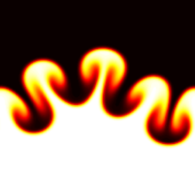
Following many two-dimensional turbulence animations, it is time to share computer code! Implementation of a vorticity-streamfunction method with a pseudo-spectral discretization + third-order Runge-Kutta for time integration (our CFD class semester project). The MATLAB code: M = 256; % number of points N = M; Lx = 2*pi; Ly = 2*pi; nu = 5e-4; % kinematic viscosity Sc = 0.7; % Schmidt number beta = 0; % meridional gradient of Coriolis parameter ar = 0.02; %random number amplitude b = 1; % mean scalar gradient CFLmax = 0.8; tend = 200; % end time x=linspace(0,Lx,M+1); x(end)=[]; dx = Lx/M; kx=[0:M/2 -M/2+1:-1]*2*pi/Lx; y=linspace(0,Ly,N+1); y(end)=[]; ky=[0:N/2 -N/2+1:-1]*2*pi/Ly; dy = Ly/N; time = 0; index_kmax = ceil(M/3); kmax = kx(index_kmax); filter = ones(M,N); filter(index_kmax+1:2*index_kmax+3,index_kmax+1:2*index_kmax+3)=0; rng(64); [u, v, omega, psi, ddx, ddy, idel2, kk, k2]=deal(zeros(M,N)); for j=1:N ddx(:,j)=1i*kx; end for i=1:M ddy(i,:)=1i*ky; end for i=1:M for j=1:N idel2(i,j)=-kx(i)^2-ky(j)^2; end end idel2=1./idel2; idel2(1,1)=0; for i=1:M for j=1:N kk(i,j)=kx(i)^2+ky(j)^2; k2(i,j)=kx(i)^2+ky(j)^2; if kk(i,j) >= 6^2 && kk(i,j) <= 7^2 % forcing kk(i,j) = -kk(i,j); end if kk(i,j) <= 2^2 kk(i,j) = 8*kk(i,j); % large-scale dissipation end end end for i=1:M for j=1:N u(i,j) = cos(2*x(i))*sin(2*y(j))+ar*rand; v(i,j) = -sin(2*x(i))*cos(2*y(j))+ar*rand; end end uhat = fft2(u); vhat = fft2(v); omegahat = ddx.*vhat - ddy.*uhat; % make vorticity phi = rand(size(u)); phihat = fft2(phi); ncid = netcdf.create(' 'CLOBBER'); dimid_x = netcdf.defDim(ncid, 'x', M); dimid_y = netcdf.defDim(ncid, 'y', N); dimid_time = netcdf.defDim(ncid, 'time', netcdf.getConstant('NC_UNLIMITED')); varid_x = netcdf.defVar(ncid, 'x', 'NC_FLOAT', [dimid_x]); varid_y = netcdf.defVar(ncid, 'y', 'NC_FLOAT', [dimid_y]); varid_u = netcdf.defVar(ncid, 'u', 'NC_FLOAT', [dimid_x, dimid_y, dimid_time]); varid_v = netcdf.defVar(ncid, 'v', 'NC_FLOAT', [dimid_x, dimid_y, dimid_time]); varid_omega = netcdf.defVar(ncid, 'vorticity', 'NC_FLOAT', [dimid_x, dimid_y, dimid_time]); varid_phi = netcdf.defVar(ncid, 'scalar', 'NC_FLOAT', [dimid_x, dimid_y, dimid_time]); varid_dissipation = netcdf.defVar(ncid, 'dissipation', 'NC_FLOAT', [dimid_x, dimid_y, dimid_time]); varid_time = netcdf.defVar(ncid, 'time', 'NC_FLOAT', [dimid_time]); netcdf.endDef(ncid); netcdf.putVar(ncid, varid_time, 0, 1, time); netcdf.putVar(ncid, varid_x, 0, M, x); netcdf.putVar(ncid, varid_y, 0, N, y); netcdf.putVar(ncid, varid_phi, [0, 0, 0], [M, N, 1], phi); netcdf.putVar(ncid, varid_u, [0, 0, 0], [M, N, 1], u); netcdf.putVar(ncid, varid_v, [0, 0, 0], [M, N, 1], v); netcdf.putVar(ncid, varid_omega, [0, 0, 0], [M, N, 1], omega); netcdf.putVar(ncid, varid_dissipation, [0, 0, 0], [M, N, 1], 0*omega); dt = 0.5*min([dx dy]); nstep = 1; while time < tend psihat = -idel2.*omegahat; uhat = ddy.*psihat; vhat = -ddx.*psihat; u = real(ifft2(uhat)); v = real(ifft2(vhat)); omegadx = real(ifft2(ddx.*omegahat)); omegady = real(ifft2(ddy.*omegahat)); facto = exp(-nu*8/15*dt*kk); factp = exp(-nu/Sc*8/15*dt*k2); r0o = -fft2(u.*omegadx+v.*omegady)+beta*vhat; r0p = -fft2(u.*real(ifft2(ddx.*phihat))+v.*real(ifft2(ddy.*phihat)))+b*vhat; omegahat = facto.*(omegahat + dt*8/15*r0o); % update omega phihat = factp.*(phihat + dt*8/15*r0p); % update phi %%%% Substep 2 psihat = -idel2.*omegahat; uhat = ddy.*psihat; vhat = -ddx.*psihat; u = real(ifft2(uhat)); v = real(ifft2(vhat)); omegadx = real(ifft2(ddx.*omegahat)); omegady = real(ifft2(ddy.*omegahat)); r1o = -fft2(u.*omegadx+v.*omegady)+beta*vhat; r1p = -fft2(u.*real(ifft2(ddx.*phihat))+v.*real(ifft2(ddy.*phihat)))+b*vhat; omegahat = omegahat + dt*(-17/60*facto.*r0o + 5/12*r1o); phihat = phihat + dt*(-17/60*factp.*r0p + 5/12*r1p); facto = exp(-nu*(-17/60+5/12)*dt*kk); factp = exp(-nu/Sc*(-17/60+5/12)*dt*k2); omegahat = omegahat.*facto; phihat = phihat.*factp; %%%% Substep 3 psihat = -idel2.*omegahat; uhat = ddy.*psihat; vhat = -ddx.*psihat; % max(max(abs(real(ifft2(1i*ddx.*uhat+1i*ddy.*vhat))))) % divergence u = real(ifft2(uhat)); v = real(ifft2(vhat)); omegadx = real(ifft2(ddx.*omegahat)); omegady = real(ifft2(ddy.*omegahat)); r2o = -fft2(u.*omegadx+v.*omegady)+beta*vhat; r2p = -fft2(u.*real(ifft2(ddx.*phihat))+v.*real(ifft2(ddy.*phihat)))+b*vhat; omegahat = omegahat + dt*(-5/12*facto.*r1o + 3/4*r2o); phihat = phihat + dt*(-5/12*factp.*r1p + 3/4*r2p); facto = exp(-nu*(-5/12+3/4)*dt*kk); factp = exp(-nu/Sc*(-5/12+3/4)*dt*kk); omegahat = omegahat.*facto; phihat = phihat.*factp; phihat = filter.*phihat; omegahat = filter.*omegahat; time = time + dt; nstep = nstep + 1; CFL = max(max(abs(u)))/dx*dt+max(max(abs(v)))/dy*dt; if mod(nstep,20)==0 phi = real(ifft2(phihat)); omega = real(ifft2(omegahat)); dissipation = 2*nu*(real(ifft2(ddx.*uhat)).^2 + real(ifft2(ddy.*uhat)).^2 + real(ifft2(ddx.*vhat)).^2 + real(ifft2(ddy.*vhat)).^2); eta = (nu^3/mean(dissipation,'all'))^0.25; subplot(221); pcolor(x,y,omega'); title('Vorticity'); shading flat; axis equal tight; colorbar; drawnow subplot(222); pcolor(x,y,phi'); title('Scalar'); shading flat; axis equal tight; colorbar; drawnow subplot(223); pcolor(x,y,dissipation'); title('Dissipation'); shading flat; axis equal tight; colorbar; drawnow subplot(224); pcolor(x,y,u); title('u-velocity'); shading flat; axis equal tight; colorbar; drawnow fprintf(1,'step = %d time = %g dt = %g CFL = %g kmax*eta = %g %g\n', nstep, time, dt, CFL, eta.*kmax, eta.*kmax/sqrt(Sc)); [~, dim_time_len] = netcdf.inqDim(ncid,dimid_time); netcdf.putVar(ncid, varid_time, [dim_time_len], [1], time); netcdf.putVar(ncid, varid_phi, [0, 0, dim_time_len], [M, N, 1], phi); netcdf.putVar(ncid, varid_u, [0, 0, dim_time_len], [M, N, 1], u); netcdf.putVar(ncid, varid_v, [0, 0, dim_time_len], [M, N, 1], v); netcdf.putVar(ncid, varid_omega, [0, 0, dim_time_len], [M, N, 1], omega); netcdf.putVar(ncid, varid_dissipation, [0, 0, dim_time_len], [M, N, 1], dissipation); netcdf.sync(ncid); end dt = CFLmax/CFL*dt; %0.0005; end netcdf.close(ncid);
226,231 次观看
Videos

Even the colorbar cannot contain its excitement about this cool animation of buoyant convection by our student Jacob Ivanov 🇺🇸! This was our CFD class term project last semester. Animation shows scaled temperature (top panel) and velocity magnitude+streamlines (bottom).
Computational Fluid Dynamics group24,980 次观看 • 1 年前
没有更多内容可加载