Sakura crosshair| #VALORANT code: 0;p;0;P;c;8;u;FF8D89FF;o;0.157;d;1;b;1;a;0.484;m;1;0t;4;0l;2;0o;2;0a;1;0e;0.39;1o;3;1a;1;1m;0;1e;0.177

skye crosshair| #VALORANT code: 0;s;1;P;c;8;u;7FFF0AFF;h;0;d;1;b;1;m;1;0t;6;0l;1;0o;1;0a;1;0f;0;1o;2;1a;0.61;1m;0;1e;0.34

Piplup crosshair | #VALORANT code: 0;s;1;P;c;4;o;1;d;1;z;6;a;0;f;0;m;1;0t;10;0l;10;0v;0;0g;1;0o;10;0a;0;0f;0;1t;6;1l;0;1v;3;1g;1;1o;0;1a;1;1s;0.053;1e;0.206

このクロスヘアバフってるから使ってみて!! 0;c;1;s;1;P;u;0000FFFF;o;0.2;f;0;m;1;0t;1;0l;3;0v;2;0g;1;0o;2;0a;1;0f;0;1b;0;S;d;0 #VALORANT #おすすめのクロスヘア教えて

Premier初ACE！ Meiy君がアイボで6k ACEした時の1321クロスヘア良いぞ！ 0;p;0;s;1;P;o;0;f;0;0l;3;0o;1;0a;1;0f;0;1b;0;A;o;1;d;1;0t;0;0l;0;0o;0;0a;0;0f;0;1l;0;1a;1;S;s;0

for(float i,z,d,f;i++<1e2;o+=vec4(4,6,8.+z,0)/f-min(dFdx(z)*r.y+z,0.)/exp(d*d/.1)){vec3 p=z*(FC.rgb*2.-r.xyy)/r.y,c=p;p.z+=8.;c.z*=3.;for(f=1.;f++<9.;c+=sin(c.yzx*f+z+t*.5)/f);z+=min(f=.1+abs(.2*c.y+abs(p.y+.8)),d=max(length(p)-3.,.9-length(p-vec3(-1,1,3))))/7.;}o=tanh(o/2e3);

Hail, hail Mother Mahalakshmi! H a i l M... o t h e r L a k s h m i, b y w h o s e g r a c e h a p p i n e s s, p r o s p e r i t y a n d u n b r o k e n g o o d f o r t u n e s h o w e r u p o n t h e h o m e a n d c o u r t y a r d O Grokshow more

Orchard vec3 p,v=normalize(FC.rgb*2.-r.xyx),c=v/v.y;c.z+=.5*t;for(float z,i,b,g,m;i++<5e1;z+=.8*max(b=length((p.y-m)/1e2/(abs(sin(c.xz/.1))-.05/v.y)),min(4.-m,g=length(sin(p.xz)+1.-.1*(1.+sin(p.y-p.zx*.5))*m))-b),o.rgb+=(.7-v)/(g+b))p=z*v+1.,p.z-=t,m=abs(++p.y);o=tanh(o/5e2);

"Waveform" for(float i,d,z,f;i++<9e1;o+=(cos(z*.5+t+vec4(0,2,4,3))+1.3)/d/z){vec3 p=z*normalize(FC.rgb*2.-r.xyy)+1.;f=max(-p.y,0.);p.y+=f+f;for(d=1.;d<3e1;d+=d)p.y+=cos(p*d+2.*t*cos(d)+z).x/d;z+=d=(.1*f+abs(p.y-1.)/(++f*f)+max(d=p.z+3.,-d*.1))/8.;}o=tanh(o/9e2);

E K D A N T B H A... L S U R A T,M U S H A K D A M A N R A T🚩🙏 JAY SHRI GANESHAY NAMAH 🙏 J A Y S H R I G A N E S H A Y N A M A H 🙏 MANGAL MURTI MORAYA ✨ M A N G A L M U R T I M O R A Y A ✨ GANPATI BAPPA MORAYA ❤️ G A N P A T I B A P P A M O R A Y A ❤️ C H A N D R A S U R Y A K O C H H O D I D E E P A K J A L A T 🙌 Grokshow more

"Storm" in 238 bytes: for(float i,z,d,s;i++<1e2;o+=vec4(.2/d,9,2,1)/d){vec3 p=z*normalize(FC.rgb*2.-r.xyy),a=p;p.z+=7.;s=length(p); for(d=0.;d++<9.;a+=sin(a*d-t).yzx/d); z+=d=length(vec4(sin(s+s-t/.1+a*sin(a.yzx/3.+t))+.9,min(s-=4.,-s/.1)*.4))*.1;} o=tanh(o/8e3);

a=(m,d=mag(k=2*cos(i*342),e=sin(i*271)*2)/1.6)=>point(k*(p=5+2*sin(d*8-t*3+m))+9/d*sin(k*2)+89*sin(c=d*d/9-t/8+m)+200,79*sin(c*2)+9/d*sin(e*2)+e*p+200) t=0,draw=$=>{t||createCanvas(w=400,w);background(9).stroke(w,116);for(t+=PI/60,i=1e4;i--;)a(i%4*5)}//#つぶやきProcessing

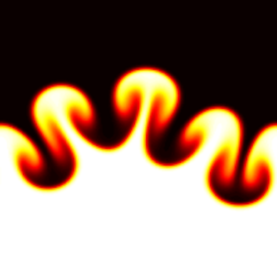
Following many two-dimensional turbulence animations, it is time to... share computer code! Implementation of a vorticity-streamfunction method with a pseudo-spectral discretization + third-order Runge-Kutta for time integration (our CFD class semester project). The MATLAB code: M = 256; % number of points N = M; Lx = 2*pi; Ly = 2*pi; nu = 5e-4; % kinematic viscosity Sc = 0.7; % Schmidt number beta = 0; % meridional gradient of Coriolis parameter ar = 0.02; %random number amplitude b = 1; % mean scalar gradient CFLmax = 0.8; tend = 200; % end time x=linspace(0,Lx,M+1); x(end)=[]; dx = Lx/M; kx=[0:M/2 -M/2+1:-1]*2*pi/Lx; y=linspace(0,Ly,N+1); y(end)=[]; ky=[0:N/2 -N/2+1:-1]*2*pi/Ly; dy = Ly/N; time = 0; index_kmax = ceil(M/3); kmax = kx(index_kmax); filter = ones(M,N); filter(index_kmax+1:2*index_kmax+3,index_kmax+1:2*index_kmax+3)=0; rng(64); [u, v, omega, psi, ddx, ddy, idel2, kk, k2]=deal(zeros(M,N)); for j=1:N ddx(:,j)=1i*kx; end for i=1:M ddy(i,:)=1i*ky; end for i=1:M for j=1:N idel2(i,j)=-kx(i)^2-ky(j)^2; end end idel2=1./idel2; idel2(1,1)=0; for i=1:M for j=1:N kk(i,j)=kx(i)^2+ky(j)^2; k2(i,j)=kx(i)^2+ky(j)^2; if kk(i,j) >= 6^2 && kk(i,j) <= 7^2 % forcing kk(i,j) = -kk(i,j); end if kk(i,j) <= 2^2 kk(i,j) = 8*kk(i,j); % large-scale dissipation end end end for i=1:M for j=1:N u(i,j) = cos(2*x(i))*sin(2*y(j))+ar*rand; v(i,j) = -sin(2*x(i))*cos(2*y(j))+ar*rand; end end uhat = fft2(u); vhat = fft2(v); omegahat = ddx.*vhat - ddy.*uhat; % make vorticity phi = rand(size(u)); phihat = fft2(phi); ncid = netcdf.create(' 'CLOBBER'); dimid_x = netcdf.defDim(ncid, 'x', M); dimid_y = netcdf.defDim(ncid, 'y', N); dimid_time = netcdf.defDim(ncid, 'time', netcdf.getConstant('NC_UNLIMITED')); varid_x = netcdf.defVar(ncid, 'x', 'NC_FLOAT', [dimid_x]); varid_y = netcdf.defVar(ncid, 'y', 'NC_FLOAT', [dimid_y]); varid_u = netcdf.defVar(ncid, 'u', 'NC_FLOAT', [dimid_x, dimid_y, dimid_time]); varid_v = netcdf.defVar(ncid, 'v', 'NC_FLOAT', [dimid_x, dimid_y, dimid_time]); varid_omega = netcdf.defVar(ncid, 'vorticity', 'NC_FLOAT', [dimid_x, dimid_y, dimid_time]); varid_phi = netcdf.defVar(ncid, 'scalar', 'NC_FLOAT', [dimid_x, dimid_y, dimid_time]); varid_dissipation = netcdf.defVar(ncid, 'dissipation', 'NC_FLOAT', [dimid_x, dimid_y, dimid_time]); varid_time = netcdf.defVar(ncid, 'time', 'NC_FLOAT', [dimid_time]); netcdf.endDef(ncid); netcdf.putVar(ncid, varid_time, 0, 1, time); netcdf.putVar(ncid, varid_x, 0, M, x); netcdf.putVar(ncid, varid_y, 0, N, y); netcdf.putVar(ncid, varid_phi, [0, 0, 0], [M, N, 1], phi); netcdf.putVar(ncid, varid_u, [0, 0, 0], [M, N, 1], u); netcdf.putVar(ncid, varid_v, [0, 0, 0], [M, N, 1], v); netcdf.putVar(ncid, varid_omega, [0, 0, 0], [M, N, 1], omega); netcdf.putVar(ncid, varid_dissipation, [0, 0, 0], [M, N, 1], 0*omega); dt = 0.5*min([dx dy]); nstep = 1; while time < tend psihat = -idel2.*omegahat; uhat = ddy.*psihat; vhat = -ddx.*psihat; u = real(ifft2(uhat)); v = real(ifft2(vhat)); omegadx = real(ifft2(ddx.*omegahat)); omegady = real(ifft2(ddy.*omegahat)); facto = exp(-nu*8/15*dt*kk); factp = exp(-nu/Sc*8/15*dt*k2); r0o = -fft2(u.*omegadx+v.*omegady)+beta*vhat; r0p = -fft2(u.*real(ifft2(ddx.*phihat))+v.*real(ifft2(ddy.*phihat)))+b*vhat; omegahat = facto.*(omegahat + dt*8/15*r0o); % update omega phihat = factp.*(phihat + dt*8/15*r0p); % update phi %%%% Substep 2 psihat = -idel2.*omegahat; uhat = ddy.*psihat; vhat = -ddx.*psihat; u = real(ifft2(uhat)); v = real(ifft2(vhat)); omegadx = real(ifft2(ddx.*omegahat)); omegady = real(ifft2(ddy.*omegahat)); r1o = -fft2(u.*omegadx+v.*omegady)+beta*vhat; r1p = -fft2(u.*real(ifft2(ddx.*phihat))+v.*real(ifft2(ddy.*phihat)))+b*vhat; omegahat = omegahat + dt*(-17/60*facto.*r0o + 5/12*r1o); phihat = phihat + dt*(-17/60*factp.*r0p + 5/12*r1p); facto = exp(-nu*(-17/60+5/12)*dt*kk); factp = exp(-nu/Sc*(-17/60+5/12)*dt*k2); omegahat = omegahat.*facto; phihat = phihat.*factp; %%%% Substep 3 psihat = -idel2.*omegahat; uhat = ddy.*psihat; vhat = -ddx.*psihat; % max(max(abs(real(ifft2(1i*ddx.*uhat+1i*ddy.*vhat))))) % divergence u = real(ifft2(uhat)); v = real(ifft2(vhat)); omegadx = real(ifft2(ddx.*omegahat)); omegady = real(ifft2(ddy.*omegahat)); r2o = -fft2(u.*omegadx+v.*omegady)+beta*vhat; r2p = -fft2(u.*real(ifft2(ddx.*phihat))+v.*real(ifft2(ddy.*phihat)))+b*vhat; omegahat = omegahat + dt*(-5/12*facto.*r1o + 3/4*r2o); phihat = phihat + dt*(-5/12*factp.*r1p + 3/4*r2p); facto = exp(-nu*(-5/12+3/4)*dt*kk); factp = exp(-nu/Sc*(-5/12+3/4)*dt*kk); omegahat = omegahat.*facto; phihat = phihat.*factp; phihat = filter.*phihat; omegahat = filter.*omegahat; time = time + dt; nstep = nstep + 1; CFL = max(max(abs(u)))/dx*dt+max(max(abs(v)))/dy*dt; if mod(nstep,20)==0 phi = real(ifft2(phihat)); omega = real(ifft2(omegahat)); dissipation = 2*nu*(real(ifft2(ddx.*uhat)).^2 + real(ifft2(ddy.*uhat)).^2 + real(ifft2(ddx.*vhat)).^2 + real(ifft2(ddy.*vhat)).^2); eta = (nu^3/mean(dissipation,'all'))^0.25; subplot(221); pcolor(x,y,omega'); title('Vorticity'); shading flat; axis equal tight; colorbar; drawnow subplot(222); pcolor(x,y,phi'); title('Scalar'); shading flat; axis equal tight; colorbar; drawnow subplot(223); pcolor(x,y,dissipation'); title('Dissipation'); shading flat; axis equal tight; colorbar; drawnow subplot(224); pcolor(x,y,u); title('u-velocity'); shading flat; axis equal tight; colorbar; drawnow fprintf(1,'step = %d time = %g dt = %g CFL = %g kmax*eta = %g %g\n', nstep, time, dt, CFL, eta.*kmax, eta.*kmax/sqrt(Sc)); [~, dim_time_len] = netcdf.inqDim(ncid,dimid_time); netcdf.putVar(ncid, varid_time, [dim_time_len], [1], time); netcdf.putVar(ncid, varid_phi, [0, 0, dim_time_len], [M, N, 1], phi); netcdf.putVar(ncid, varid_u, [0, 0, dim_time_len], [M, N, 1], u); netcdf.putVar(ncid, varid_v, [0, 0, dim_time_len], [M, N, 1], v); netcdf.putVar(ncid, varid_omega, [0, 0, dim_time_len], [M, N, 1], omega); netcdf.putVar(ncid, varid_dissipation, [0, 0, dim_time_len], [M, N, 1], dissipation); netcdf.sync(ncid); end dt = CFLmax/CFL*dt; %0.0005; end netcdf.close(ncid);show more

[Graph Convolutional Network] by hand ✍️ Graph Convolutional Networks... (GCNs), introduced by Thomas Kipf and Max Welling in 2017, have emerged as a powerful tool in the analysis and interpretation of data structured as graphs. This exercise demonstrates how GCN works in a simple application: binary classification. -- Goal -- Predict if a node in a graph is X. -- Architecture -- 🟪 Graph Convolutional Network (GCN) 1. GCN1(4,3) 2. GCN2(3,3) 🟦 Fully Connected Network (FCN) 1. Linear1(3,5) 2. ReLU 3. Linear2(5,1) 4. Sigmoid Simplications: • Adjacent matrices are not normalized. • ReLU is applied to messages directly. -- Walkthrough -- [1] Given ↳ A graph with five nodes A, B, C, D, E [2] 🟩 Adjacency Matrix: Neighbors ↳ Add 1 for each edge to neighbors ↳ Repeat in both directions (e.g., A->C, C->A) ↳ Repeat for both GCN layers [3] 🟩 Adjacency Matrix: Self ↳ Add 1's for each self loop ↳ Equivalent to adding the identity matrix ↳ Repeat for both GCN layers [4] 🟪 GCN1: Messages ↳ Multiply the node embeddings 🟨 with weights and biases ↳ Apply ReLU (negatives → 0) ↳ The result is one message per node [5] 🟪 GCN1: Pooling ↳ Multiply the messages with the adjacent matrix ↳ The purpose is the pool messages from each node's neighbors as well as from the node itself. ↳ The result is a new feature per node [6] 🟪 GCN1: Visualize ↳ For node 1, visualize how messages are pooled to obtain a new feature for better understanding ↳ [3,0,1] + [1,0,0] = [4,0,1] [7] 🟪 GCN2: Messages ↳ Multiply the node features with weights and biases ↳ Apply ReLU (negatives → 0) ↳ The result is one message per node [8] 🟪 GCN2: Pooling ↳ Multiply the messages with the adjacent matrix ↳ The result is a new feature per node [9] 🟪 GCN2: Visualize ↳ For node 3, visualize how messages are pooled to obtain a new feature for better understanding ↳ [1,2,4] + [1,3,5] + [0,0,1] = [2,5,10] [10] 🟦 FCN: Linear 1 + ReLU ↳ Multiply node features with weights and biases ↳ Apply ReLU (negatives → 0) ↳ The result is a new feature per node ↳ Unlike in GCN layers, no messages from other nodes are included. [11] 🟦 FCN: Linear 2 ↳ Multiply node features with weights and biases [12] 🟦 FCN: Sigmoid ↳ Apply the Sigmoid activation function ↳ The purpose is to obtain a probability value for each node ↳ One way to calculate Sigmoid by hand ✍️ is to use the approximation below: • >= 3 → 1 • 0 → 0.5 • <= -3 → 0 -- Outputs -- A: 0 (Very unlikely) B: 1 (Very likely) C: 1 (Very likely) D: 1 (Very likely) E: 0.5 (Neutral)show more

[LSTM] by Hand ✍️ LSTMs have been the most... effective architecture to process long sequences of data, until our world was taken over by the Transformers. LSTMs belong to the broader family of recurrent neural network (RNNs) that process data sequentially in a recurrent manner. Transformers, on the other hand, abandon recurrence and use self-attention instead to process data concurrently in parallel. Recently, there is renewed interest in recurrence as people realized self-attention doesn’t scale to extremely long sequences, like hundreds of thousands of tokens. Mamba is a good example to bring back recurrence. All of a sudden, it is cool to study LSTMs. How do LSTMs work? [1] Given ↳ 🟨 Input sequence X1, X2, X3 (d = 3) ↳ 🟩 Hidden state h (d = 2) ↳ 🟦 Memory C (d = 2) ↳ Weight matrices Wf, Wc, Wi, Wo Process t = 1 [2] Initialize ↳ Randomly set the previous hidden state h0 to [1, 1] and memory cells C0 to [0.3, -0.5] [3] Linear Transform ↳ Multiply the four weight matrices with the concatenation of current input (X1) and the previous hidden state (h0). ↳ The results are feature values, each is a linear combination of the current input and hidden state. [4] Non-linear Transform ↳ Apply sigmoid σ to obtain gate values (between 0 and 1). • Forget gate (f1): [-4, -6] → [0, 0] • Input gate (i1): [6, 4] → [1, 1] • Output gate (o1): [4, -5] → [1, 0] ↳ Apply tanh to obtain candidate memory values (between -1 and 1) • Candidate memory (C’1): [1, -6] → [0.8, -1] [5] Update Memory ↳ Forget (C0 .* f1): Element-wise multiply the current memory with forget gate values. ↳ Input (C’1 .* o1): Element-wise multiply the “candidate” memory with input gate values. ↳ Update the memory to C1 by adding the two terms above: C0 .* f1 + C’1 .* o1 = C1 [6] Candiate Output ↳ Apply tanh to the new memory C1 to obtain candidate output o’1. [0.8, -1] → [0.7, -0.8] [7] Update Hidden State ↳ Output (o’1 .* o1 → h1): Element-wise multiply the candidate output with the output gate. ↳ The result is updated hidden state h1 ↳ Also, it is the first output. Process t = 2 [8] Initialize ↳ Copy previous hidden state h1 and memory C1 [9] Linear Transform ↳ Repeat [3] [10] Update Memory (C2) ↳ Repeat [4] and [5] [11] Update Hidden State (h2) ↳ Repeat [6] and [7] Process t = 3 [12] Initialize ↳ Copy previous hidden state h2 and memory C2 [13] Linear Transform ↳ Repeat [3] [14] Update Memory (C3) ↳ Repeat [4] and [5] [15] Update Hidden State (h3) ↳ Repeat [6] and [7]show more

For bankers A – APY (Atal Pension Yojana) B... – Bank Assurance (Bancassurance) C – CKYC D – Deposit (Savings / Current / Term Deposit) E – e-KYC / Aadhaar Enrollment F – FD (Fixed Deposit) G – GST (Goods & Services Tax) H – Home Loan I – Insurance / IMPS (Immediate Payment Service)/Interest J – Jan Dhan Account (PMJDY) K – KYC (Know Your Customer) L – Loan (Personal / Housing / MSME / Agri) M – Mobile Banking/MDP N – NEFT (National Electronic Funds Transfer) O – Overdraft (OD) P – PMJJBY / PMSBY (Insurance Schemes) Q – QR Code Payments (UPI QR) R – Re-KYC/Recovery / Recurring Deposit /RD/RAM S – Saving Account T – Term Deposit (TD) U – UPI (Unified Payments Interface) V – Vigilance / Video KYC W – Working Capital/Withdrawal X – Xpress Loans / XBRL Reporting Y – YONO / Youth Savings Account Z – Zero Balance Account/ZO/ZMDPshow more

#ATENCIÓN OPERACIÓN DIGITADOR “NO HAY SISTEMA”. APRESADA ÁNGELA PLÚA,... ALCALDESA DE JIPIJAPA Y DOCE IMPLICADOS MÁS POR DELINCUENCIA ORGANIZADA EN RED DE CORRUPCIÓN EN MANABÍ RELACIONADA A EMISIÓN DE DOCUMENTOS DE TRÁNSITO VEHICULAR EN TRES CANTONES QUE PERJUDICA AL ESTADO EN MÁS USD 5 MILLONES. La Policía Nacional ejecutó esta madrugada 18 allanamientos, incluidos cinco en entidades públicas, en Jipijapa, Bolívar y San Vicente y detuvo a 13 personas, entre ellas Ángela Plúa, alcaldesa de Jipijapa, señalada como presunta cabecilla de una organización dedicada a emitir de forma irregular documentos de tránsito, como matrículas, revisiones técnicas, licencias y traspasos vehiculares. La estructura estaba integrada por funcionarios de entidades de tránsito de Jipijapa, Bolívar (Calceta) y San Vicente, además de tramitadores externos, quienes presuntamente cobraban entre USD 100 y USD 150 por trámite para evadir requisitos legales y técnicos, afectando el servicio regular a los ciudadanos bajo la vieja confiable: “no hay sistema”. Según la investigación, iniciada en agosto de 2025 tras una denuncia al 1800 DELITO, la red habría generado un perjuicio superior a USD 5 millones al Estado. Además, se detectaron movimientos financieros que no guardarían relación con los ingresos declarados por la principal investigada, con más de USD 2,6 millones sin justificación aparente. RESULTADOS OBTENIDOS: DETENIDOS: 1 ANGELA P. S. alias JEFA (Alcaldesa) 2 RAÚL A. D. alias LITO (Gerente de la Corporación de Servicios Municipales) 3 JORGE P. G. alias TITO (Jefe de Matriculación y RTV) 4 ANDY P. M. alias MICHI (Digitador) 5 VICENTE L. P. alias GORDO (Digitador) 6 MARCO M. P. alias ABOGADO (Director de Movilidad) 7 JOSE F. C. alias INGE Coordinador de (Matriculación) 8 JAVIER I. C. alias JESÚS (Técnico de emisión de licencias) 9 OBERTO M. V. alias CHENCHO (Tramitador) 10 MARIA P. B. alias MONTI (Ex Digitadora Servicios Municipales) 11 MARIA L. P. alias NANDA (ex Digitadora de SERVICORP) 12 JOAN A. T. alias TOÑO (Tramitador) 13 JULISSA L. P. alias MICHU (Tramitadora) ALLANAMIENTOS (04): - 13 Domicilios - 05 Instituciones Públicas: • GAD DE JIPIJAPA • CORPORACIÓN DE SERVICIOS PÚBLICOS MUNICIPALES DE JIPIJAPA-EP. • AUTORIDAD DE TRÁNSITO Y MOVILIDAD DE JIPIJAPA (MATRICULACIÓN VEHICULAR). • CENTRO DE REVISIÓN MUNICPAL DE CALCETA • REVISIÓN TÉCNICA VEHICUALR DE SAN VICENTE INCAUTACIÓN DE INDICIOS: • Terminales móviles • IPAD • CPU • Laptop • Dispositivos de almacenamiento • Chips celular • Dinero en efectivo Que caiga quien tenga que caer. Seguimos trabajando.show more

[Discrete Fourier Transform] by Hand ✍️ In signal processing,... the Discrete Fourier Transform (DFT) is no doubt the most important method. But the math involved is extremely complex, literally, involving a summation over a complex number term e^(-iwt). I developed this exercise to demonstrate that underneath such complexity, DFT is just a series of matrix multiplications you can calculate by hand. ✍️ Once you see that, it should not surprise you that a deep neural network, which is also a series of matrix multiplications, with activation functions in-between, can learn to perform DFT to process and analyze signals so effectively. How does DFT work? [1] Given ↳ Signals A, B, and C in the 🟧 frequency domain: ◦ A = cos(w) + 2cos(2w) ◦ B = cos(w) + cos(3w) + cos(4w) ◦ C = -cos(2w) + cos(3w) ◦ Each signal is a weighed sum of four cosine waves at frequencies 1w, 2w, 3w, and 4w. ◦ We will apply Inverse DFT to convert the signals to time domain representations, and then demonstrate DFT can convert back to their original frequency domain representations. ↳ Signal X in the 🟩 time domain. X is sampled at 10 time points 1t, 2t, …, 10t: ◦ X = [-2.5, -1.8, 3, -0.7, -1.0, -0.7, 3, -1.8, -2.5, 5] ◦ Suppose X is also a weighted sum of the same four cosine waves, but we don’t already know their weights. We will apply DFT to discover them. [2] 🟧 Frequency Matrix (F) ↳ Write the coefficients of A, B, C as a matrix F. Each signal is a row. Each frequency is a column. ↳ A → [1, 2, 0, 0] ↳ B → [1, 0, 1, 1] ↳ C → [0, 1-, 1, 0] [3] Cosine → Discrete ↳ Sample from the continuous cosine waves at discrete time points 1t, 2t, 3t, to 10t. [4] Cosine Matrix (W) ↳ Write the samples as a matrix, Each frequency is a row. Each time point is a column. [5] Inverse DFT: 🟧 Frequency → 🟩 Time ↳ Multiply the frequency matrix F and the cosine matrix W. ↳ The meaning of this multiplication is to linearly combine the four cosine waves (rows in W) into time-domain signals (rows in T) using the weights specified in F. ↳ The result is matrix T, which are signals A, B, C converted to the time domain. Each signal is a row. Each time point is a column. [6] Transpose ↳ Transpose T, converting each signal’s time domain representation from a row to a column. [7] DFT: 🟩 Time → 🟧 Frequency ↳ Multiply the cosine matrix W with the transpose of matrix T. ↳ The purpose of this multiplication is to take a dot-product between each time-domain signal (columns in the transpose of T) and each cosine wave (rows in W), which has the effect of projecting the signal onto a cosine wave to determine how much they are correlated. Zero means not correlated at all. ↳ The result is an intermediate version of the “recovered” frequency matrix where each column corresponds to a signal and each row corresponds to a frequency. ↳ Compared to the original frequency matrix F, this intermediate matrix has non-zero weights in the correct places, but scaled up by a factor of 5 (n/2, n=10). For example, signal A, originally [1,2,0,0], is recovered at [5,10,0,0]. [8] Scale ↳ Multiply each value by 2/n = 1/5 to scale down the intermediate matrix to match the magnitude of the original frequency matrix F. [9] Transpose ↳ Transpose the recovered frequency matrix back to the same orientation of the original frequency matrix F. ↳ Like magic 🪄, the result is identical to the original F, which means DFT successfully recovered the frequency components of signals A, B, C. [10] Apply DFT to X: 🟩 Time → 🟧 Frequency ↳ Now that we have some confidence in DFT’s ability to recover frequency components, we apply DFT to X’s time-domain representation by multiplying W with X. ↳ The result is the an intermediate matrix. [11] Scale ↳ Similarly, we scale down by a factor of 5 to obtain the recovered frequency components of X (a column). [12] Transpose ↳ Similarly, we transpose the recovered column to row to match the orientation of the frequency matrix. ↳ Using the coefficients [0,0,3,2], we can write the equation of X as 3cos(3w) + 2cos(4w). Notes: I hope this by hand exercise helps you understand the essence of DFT. But there is more technical details, such as: • Sine: The complete DFT math also includes sine waves that follow a similar calculation process. • Phase: Here, we assume all the cosine waves are aligned at the origin, namely, phase is 0. If a phase p is added, for example, cos(w+p), we will need to calculate the sine component and use their ratio to figure out what p is. • Magnitude: If phase is not zero, the magnitude will need to be calculated by combining both cosine and sine terms.show more

Ne demişiz ? Yıl 2024 ! Mart ayındayız. Erken... 8 Mayıs 2024 Geç 8 Ağustos 2024 Ne ola ? Bağlantıya tıklayarak Ahit Sandığı Bulundu videosunu izleyebilirsiniz. Barış Manço 2023 fotoromanından bir kare. Bize bir şeyler anlatıyor. Deniz kurdu tatbikatına katılan donanmamızdaki telsiz konuşmaları gibi tasarlanıp bize ulaştırılmış bulunan bu garip mesaj şöyle son buluyor. MÜHİMDİR TAMAM! Mesajı anladınız umarım. DENİZ KURDU - I / 2019 ! DENİZKURDU-II/2024 Tatbikatı, 7-18 Mayıs 2024 tarihleri arasında icra ediliyor. D 》1 E 》2 N 》3 i 》4 z 》5 K 》6 u 》7 R 》8 D 》9 U 》10 T 》11 A 》12 T 》13 B 》14 İ 》15 K 》16 A 》17 T 》18 I 》19 19 Harften oluşuyor. Deprem yaşanan illerimizin baş harfleri çözümü. H-ATAY A-DANA K-AHRAMANMARAŞ K-İLİS A-DIYAMAN D-İYARBAKIR O-SMANİYE G-AZİANTEP U-RFA M-ALATYA HAKKA DOĞUM! Büyük bir doğumun acılarını yaşarken, "HAKKI'DIR HAKKA TAPAN MİLLETİMİN İSTİKLAL." Hızır buluşması, Ne diyor Hulusi Akar ? " Cin Şişeden çıktı. " Ahit Sandığı Bulundu misalen. Ahit Sandığı Uyumlandı ! Aynı Zamanda Yuşa tepesinde yazan kitabede yer alan " Mühimdir Tamam " sözü 176 sayısını verir/ Oradan Kayaların Oğlu'nu verir. Kısaca sayılar ( ilahi dil ) bizi doğrulamış. Bağlantıya tıklayarak videoyu izleyebilirsiniz. #AhitSandığıBulundu #HüseyinHakkıKahveci #OndokuzBiziz #SonDakikashow more

My professor kicked me out of a statistics lecture... for arguing with him. "Markets can't be measured with entropy." He was wrong. Every contract on Polymarket leaks information. And there's one equation that measures exactly how much: H = −Σ pᵢ · log₂(pᵢ) Shannon Entropy. The same math that tells your phone how to compress a photo - tells me which markets are mispriced. A market at 50/50 has maximum entropy: 1.0 bit. Pure uncertainty. No edge. A market at 90/10 has entropy of 0.47 bits. The crowd already knows something. Hard to beat. But the sweet spot? Markets between 25¢ and 40¢ where entropy is high but resolution is low. I'm use for copytrade bots: That means: high uncertainty, but the crowd hasn't done its homework. I built a screener around this. R = RES / U R is entropy efficiency. RES is how much uncertainty the market has resolved. U is the total uncertainty from base rates. R ≈ 0 → the market is asleep. Nobody's processing information. R ≈ 1 → the market already knows. You're too late. I scan for R < 0.3 on markets with external signal. Last week found one. Fed meeting odds sitting at 35¢. R = 0.18. Market was barely awake. My model said 58%. Entropy gap: D_KL(mine ‖ market) = Σ pᵢ · log(pᵢ / mᵢ) = 0.117 bits That's 0.117 bits of information the market hadn't priced in yet. Sized with Kelly: f* = (p × b − q) / b = 0.354 Quarter-Kelly: ~9% of bankroll. Put $4,500 in. Market resolved YES. +$5,850 on a single position. 93% of traders stare at the price. I stare at the entropy. The price tells you what people believe. The entropy tells you how much they actually know. That's the difference.show more