Video yükleniyor...

Video Yüklenemedi

Ana Sayfaya Dön

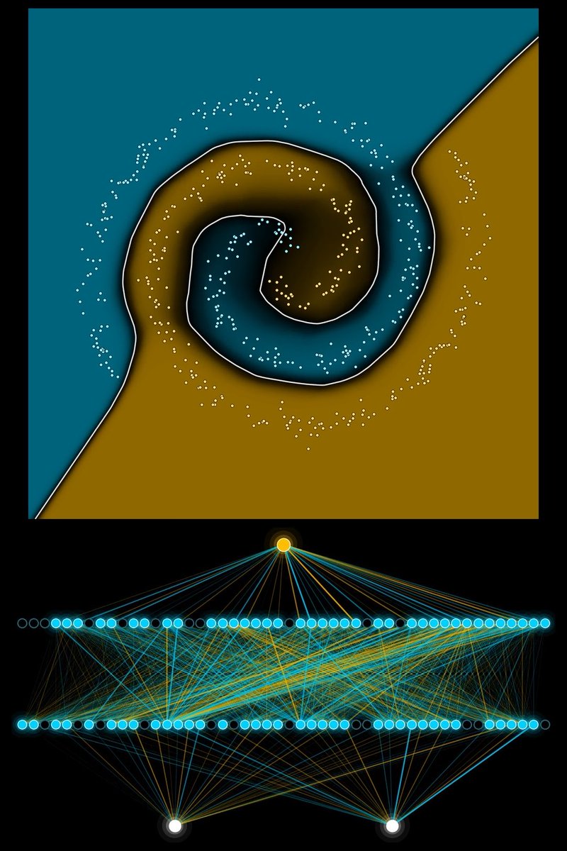
➡️Machine Learning from Scratch, part 51: dropout. At every training step each hidden neuron flips its own coin and about half of them are switched off, a new random half every step. No neuron can lean on its neighbours, so the knowledge spreads over many neurons, and only patterns...

14,500 görüntüleme • 4 gün önce •via TikTok

0 Yorum

Yorum bulunmuyor

Orijinal gönderinin yorumları burada görünecek

Benzer Videolar

➡️ Part 9 of learning ML code from scratch Six weights, one wrong answer, and not one of them knows it was at fault. Backpropagation is how they find out. Two questions guide the video: what even is backpropagation, and why do models need it? Step 1, the forward pass. Two numbers go into a tiny network, run through a hidden layer, and one number comes out. Ours says 0.700. We wanted 1.0, so square the difference and the loss is 0.09. That single number is how wrong the model is. Step 2, the question. Six weights produced that answer together. Which of them is to blame, and by how much? Step 3, the one idea. Change a single weight by a tiny amount and watch the error move. How much the error changes per unit of weight is the gradient of that weight. In the video you can see it happen: the weight wobbles and the error bar answers. Step 4, the shortcut. Every weight running into the same neuron starts from one shared number, the blame of that neuron. Multiply that blame by the value each weight carried and you have its gradient. One blame, computed once, and every weight into that neuron gets its own gradient from it. That is why backpropagation is fast enough to train anything at all. Step 5, backwards. The blame starts at the output and every layer hands its share to the layer in front of it, back through the same network the data came forward through. It goes layer by layer, and inside one layer every neuron is done together. Step 6, the update. The optimizer moves every weight against its own gradient, the whole weight matrix in one go, so no weight waits for its turn. All six gradients here are negative, so all six weights go up. After one step the answer reads 0.769. After sixty it reads 0.968 and the error is down to 0.001. The honest part: every gradient in the video was checked against the measured change of the error. Move that one weight, see what the error does, divide. Backprop and the measurement agree to nine decimal places, otherwise nothing would have rendered. #machinelearning #backpropagation #neuralnetworks #python #coding

MachineLearningToGo

210,300 görüntüleme • 1 ay önce

➡️ Machine Learning from Scratch, part 47: the Hopfield network. In 1982 the physicist John Hopfield described a network that works as a memory, and 42 years later this work was part of the Nobel Prize in Physics. Each neuron is one pixel that is either on or off, and every neuron is connected to every other neuron, so 100 pixels need 4,950 connections. There are no layers: signals go back and forth until the network settles. Each neuron takes a weighted sum of its inputs and switches on if the sum is positive, off if it is negative. Storing a picture is simple: for every pair of pixels with the same colour the connection gets stronger, otherwise weaker. Every stored picture becomes a valley in the energy landscape, and no switch can ever raise the energy, so a noisy picture rolls downhill into the nearest stored memory. The code (hopfield.py, 16 lines of numpy, pictures in pics.txt) stores three 10 x 10 pictures, a heart, a house and a smiley, and flips 30 of the 100 pixels in each. After a single pass over all neurons all three come back exactly; the energy of the heart falls from -6.90 to -48.90, the energy of the stored heart. With 100 neurons and random patterns (10 flipped pixels, 20 runs) it recalls 5 patterns every time, 10 patterns in 94.5 % of the cases, 14 in 68 %, 20 in about one in four (24 %) and 30 in 1 %. Honest notes: the weights are kept as whole numbers (100 times the Hebb weight), so a sum of exactly zero switches the neuron on, as the rule says. The landscape in the video is a picture of the idea; the valley floors and the height of the rolling ball are the real energies from the run. #machinelearning #ai #coding #neuralnetworks #nobelprize

MachineLearningToGo

11,900 görüntüleme • 12 gün önce

Dropout by hand ✍️ ~ 10 steps walkthrough below Dropout is the simplest trick in deep learning that actually works: during training you randomly switch neurons off, so the network cannot lean on any one of them. It is two lines of code and almost nobody has worked through what those lines do to the numbers. So I drew and calculated one entirely by hand. Goal: train one pass through a small network with two dropout layers, then run inference with dropout switched off. The network: Linear(2,4), ReLU, Dropout(0.5), Linear(4,3), ReLU, Dropout(0.33), Linear(3,2). = 1. Given = A training set of two examples, X1 and X2, and the weight matrices for all three linear layers. = 2. Draw the first random numbers = Let us draw 4 random numbers, one per neuron in the first hidden layer. Above 0.5 we keep (◯), below we drop (╳). Here that gives [◯, ╳, ◯, ╳]. = 3. Build the first dropout matrix = We turn that pattern into a diagonal matrix. The scaling factor is 1/(1-p) = 2, so a kept neuron gets 2 and a dropped one gets 0. Multiplying by it does both jobs at once: it deletes the 2nd and 4th neurons and doubles the two that survive. = 4. Draw the second random numbers = Let us do it again for the 3 neurons in the next layer, this time against p = 0.33. The result is [◯, ◯, ╳]. = 5. Build the second dropout matrix = We set the diagonal to 1.5 where kept and 0 where dropped. Only the 3rd neuron goes. = 6. Feed forward = Let us run the whole thing top to bottom: one matrix multiplication per layer, ReLU setting the negatives to zero, and the two dropout matrices doing their work in between. The outputs Y come out at the bottom. = 7. MSE loss gradients = We compare Y against the targets Y', subtract, and multiply each element by 2. That is the whole gradient of the mean squared error. = 8. Update the weights = Let us push those gradients back through the network and update the weights (marked in light red). = 9. Deactivate dropout = Training is over, so we set both dropout matrices to the identity. Every neuron is back, and nothing is scaled. = 10. Feed forward again = One more pass, this time on unseen data, to make the prediction. You have just trained and run a network with dropout by hand. ✍️ The outputs: Training outputs Y = [-6, 9; 13, 4] Loss gradients = [-4, 4; 6, -2] Inference outputs = [13, 13; 4, 3] 💾 Save this post! #AIbyHand #Dropout #DeepLearning #NeuralNetworks

Tom Yeh

14,442 görüntüleme • 3 ay önce

➡️ ML news part 1 An AI just fixed another AI by rewriting its weights directly, without any training. Machine Learning News, part 1: weight space programming. What is new, and why it matters. Until now, the weights of a neural network were set by training, and reading them took special tools built for that one job. A new report from researchers at MIT CSAIL shows that a general AI model, here GPT-6 Astra used as it is, can read and write those weights directly as plain lists of numbers. Test 1, reading. The model was given only the 17,253 weights of four small game playing networks (Breakout, Pong, Pac-Man, Freeway) and named the right game for all four. Test 2, writing. Without any data, loss or gradients, it wrote networks for three MinAtar games, and all three beat networks trained with PPO for 100 million steps. In Breakout it scored 517.4 points, against 25.3 after 500 million training steps. Test 3, repairing. The small open language model Qwen3.5-0.8B ran into its length limit on 93 percent of MATH-500 answers because it got stuck in loops. The model traced the loop to one direction written by the MLPs of layers 15 and 19 and removed it. That changed 131,072 weights, which is 0.016 percent of the model. MATH-500 went from 7.9 to 48.1 percent, IFEval from 21.0 to 62.3 percent, GSM8K from 13.8 to 67.1 percent, all with no training. The edit was chosen with a budget of 50 trial runs on practice problems, and the test sets were never seen. To be fair, the authors say the fix removed an obstacle and added no new ability, and on another small model it brought no improvement. This is an early report and not yet peer reviewed. Source: Takehi, Teoh, Zhang, Khattab (MIT CSAIL), "Sparks of Weight-Space Programming", blog post, November 2, 2026, (early report, not peer reviewed). Screenshots from the report are shown as quotes. Model names are given only to name the source. #machinelearning #ai #claude #neuralnetworks #llm

MachineLearningToGo

55,800 görüntüleme • 9 gün önce

➡️ Machine Learning from Scratch, part 31: the transformer. A transformer turns every token into a list of numbers, adds its position, and then lets every token look at the others. That step is called attention: each token has a query (what am I looking for), a key (what do I contain) and a value (what I pass on). The better a query matches a key, the more of that value flows in. Real transformers repeat this in many layers with several attention heads each. The design comes from the 2017 Google paper "Attention Is All You Need" by Ashish Vaswani and colleagues, first used for translation. A large language model is a transformer trained to predict the next token, again and again, on a huge amount of text. Our own run, nothing downloaded. attention.py is one self-attention layer in 16 lines of numpy. Every word gets a query, a key and a value of 8 numbers, starting random, trained from scratch with hand-written backpropagation on 192 made-up sentences like "the dog ate the carrot because it was hungry". The task: find out which pet "it" means. On 64 new test sentences "it" puts 99.95 percent of its attention on the right word on average (the lowest single sentence gets 99.9 percent; the program prints this as 100%). Before training it was 10 percent, spread evenly. The cat sentence from the video is one of the test sentences. Honest notes: our task is easy on purpose. Every sentence has exactly one pet, so "it" only has to learn to look for pets, and it learns that within the first pass. Real sentences with two candidates need more context, which is what many layers are for. Our small version has no positions, no scaling, no mask, one head, and only "it" asks a question. Every word of the test sentences also appears in training; the combinations are new. The 3D space in the video shows the real keys of our model, projected to three axes (two of them stretched so you can see them). The stacked layers are a sketch. #machinelearning #ai #transformer #python #llm

MachineLearningToGo

79,900 görüntüleme • 1 ay önce

➡️ Quantitative Finance from Scratch, part 45: Statistical Arbitrage. The arbitrage from the last part was a profit without any risk. Statistical arbitrage is the practical version: many small bets that can each lose, but win on average. One of the best known and simplest forms is pairs trading: two stocks in the same business that move together. The gap between them, the spread = P_A − β · P_B (P_A price of stock A, P_B price of stock B, β the hedge ratio), keeps coming back to its average. That is the edge: the trade treats this return almost like a law, so the further the spread moves away, the more it should come back, and that way back is the profit. The rule: z = (spread − average) / standard deviation. When z reaches +2 or −2, you sell the expensive stock, buy the cheap one, and close both when the gap is back at its average. Because one stock is long and the other short, a move of the whole market mostly cancels out. News about one company can still hit a single pair, so funds make many such trades at once, and the surprises average out. The big risks: the link between two stocks can break for good, for example after a merger, and when many funds hold the same trades, they can all lose at once. The code (statarb_reel.py, 16 lines of plain Python without packages) is general on purpose: the spread from two prices and the hedge ratio, the z score, and the signal that sells the expensive stock and buys the cheap one at two standard deviations and closes at the average. If you want to go deeper, the link to my website is in my bio. #quantfinance #statisticalarbitrage #pairstrading #meanreversion #python Education only, not financial advice.

QuantFinanceToGo

37,500 görüntüleme • 3 gün önce