Video yükleniyor...

Video Yüklenemedi

Ana Sayfaya Dön

A neural network can begin as a flat sheet and learn the shape of hidden data A self-organizing map turns learning into geometry. Each data point pulls one winning neuron toward it, but nearby neurons move too, and so the whole lattice bends without losing its neighborhood structure. The...

129,934 görüntüleme • 3 ay önce •via X (Twitter)

0 Yorum

Yorum bulunmuyor

Orijinal gönderinin yorumları burada görünecek

Benzer Videolar

What if Your Neural Network Was Forced to Obey Physics? Physics-Informed Neural Networks (PINNs) are neural networks trained to satisfy a differential equation by building the PDE residual directly into the loss. They emerged from a very practical problem...classical PDE pipelines can be brilliant, but they often demand heavy discretization work (meshes, stencils, stability tuning), and the method you build is usually tied to one geometry and one solver setup. A PINN flips the workflow by representing the solution itself as a smooth function uᵩ(x,t) and enforcing the physics everywhere you choose to sample the domain. People often meet PINNs in the least helpful way...via a flashy solution plot, and almost no explanation of what was enforced to get it. In this series we keep the enforcement visible. We pick a differential equation, represent the unknown solution as a flexible function, measure how well that function satisfies the equation across the domain, and train it to reduce that mismatch everywhere we sample. A normal neural net learns from labels...you give it inputs and target outputs. A PINN learns from a differential equation...you give it inputs (x,t) and it gets punished whenever its output fails the PDE. By punish we mean that the loss increases when the mismatch is large we reward it if the loss decreases as the mismatch gets smaller. The network isn’t replacing physics, it’s becoming a flexible function that is forced to satisfy the same calculus you’d impose on any candidate solution. The math breakdown: We start with a PDE we want to solve on a domain Ω. Write it as uₜ(x,t) + N(u(x,t), uₓ(x,t), uₓₓ(x,t), …) = 0 for (x,t) in Ω A PINN replaces the unknown function u with a neural network output uᵩ(x,t) Now define the physics residual by plugging uᵩ into the PDE rᵩ(x,t) = ∂uᵩ/∂t + N(uᵩ, ∂uᵩ/∂x, ∂²uᵩ/∂x², …) If uᵩ were an exact solution, we would have rᵩ(x,t) = 0 everywhere. We may also have data points (xᵢ,tᵢ,uᵢ) from measurements or a known initial condition. The training objective is just a weighted sum of squared errors L(ᵩ) = L_data(ᵩ) + λ L_phys(ᵩ) + L_bc/ic(ᵩ) with L_data(ᵩ) = meanᵢ |uᵩ(xᵢ,tᵢ) − uᵢ|² L_phys(ᵩ) = meanⱼ |rᵩ(xⱼ,tⱼ)|² where (xⱼ,tⱼ) are the collocation points in Ω L_bc/ic(ᵩ) = penalties enforcing boundary conditions and initial conditions The key technical step is that the derivatives inside rᵩ are computed by automatic differentiation ∂uᵩ/∂t, ∂uᵩ/∂x, ∂²uᵩ/∂x², … So we can differentiate the total loss L(ᵩ) with respect to ᵩ and train with gradient descent. This is the whole idea behind PINNs. Learn a function, but make the PDE part of the loss, so the network is trained to be a solution, not just a curve-fitter. In the render, the main 3D surface is the network’s current guess uᵩ(x,t), drawn as a living sheet over the (x,t) plane. Hovering above is the neural scaffold...a visible graph of feature nodes and connections. The bright tension threads are the physics residual rᵩ(x,t): each thread tethers a collocation bead on the sheet up to the scaffold, and it thickens and brightens exactly where |rᵩ| is large (color encodes the sign). As training runs, those threads go slack across the domain not because we hid the error, but because the network has actually been pushed toward rᵩ(x,t) ≈ 0. #PINNs #PhysicsInformedNeuralNetworks #ScientificMachineLearning #PDE #DifferentialEquations #Optimization #MachineLearning #AppliedMath #ComputationalPhysics

Mathelirium

17,285 görüntüleme • 2 ay önce

Lecture 1 on Physics-Informed Neural Networks: A Mini-Series Physics-Informed Neural Networks (PINNs) are neural networks trained to satisfy a differential equation by building the PDE residual directly into the loss. They emerged from a very practical problem...classical PDE pipelines can be brilliant, but they often demand heavy discretization work (meshes, stencils, stability tuning), and the method you build is usually tied to one geometry and one solver setup. A PINN flips the workflow by representing the solution itself as a smooth function uᵩ(x,t) and enforcing the physics everywhere you choose to sample the domain. People often meet PINNs in the least helpful way...via a flashy solution plot, and almost no explanation of what was enforced to get it. In this series we keep the enforcement visible. We pick a differential equation, represent the unknown solution as a flexible function, measure how well that function satisfies the equation across the domain, and train it to reduce that mismatch everywhere we sample. A normal neural net learns from labels...you give it inputs and target outputs. A PINN learns from a differential equation...you give it inputs (x,t) and it gets punished whenever its output fails the PDE. By punish we mean that the loss increases when the mismatch is large we reward it if the loss decreases as the mismatch gets smaller. The network isn’t replacing physics, it’s becoming a flexible function that is forced to satisfy the same calculus you’d impose on any candidate solution. The math breakdown: We start with a PDE we want to solve on a domain Ω. Write it as uₜ(x,t) + N(u(x,t), uₓ(x,t), uₓₓ(x,t), …) = 0 for (x,t) in Ω A PINN replaces the unknown function u with a neural network output uᵩ(x,t) Now define the physics residual by plugging uᵩ into the PDE rᵩ(x,t) = ∂uᵩ/∂t + N(uᵩ, ∂uᵩ/∂x, ∂²uᵩ/∂x², …) If uᵩ were an exact solution, we would have rᵩ(x,t) = 0 everywhere. We may also have data points (xᵢ,tᵢ,uᵢ) from measurements or a known initial condition. The training objective is just a weighted sum of squared errors L(ᵩ) = L_data(ᵩ) + λ L_phys(ᵩ) + L_bc/ic(ᵩ) with L_data(ᵩ) = meanᵢ |uᵩ(xᵢ,tᵢ) − uᵢ|² L_phys(ᵩ) = meanⱼ |rᵩ(xⱼ,tⱼ)|² where (xⱼ,tⱼ) are the collocation points in Ω L_bc/ic(ᵩ) = penalties enforcing boundary conditions and initial conditions The key technical step is that the derivatives inside rᵩ are computed by automatic differentiation ∂uᵩ/∂t, ∂uᵩ/∂x, ∂²uᵩ/∂x², … So we can differentiate the total loss L(ᵩ) with respect to ᵩ and train with gradient descent. This is the whole idea behind PINNs. Learn a function, but make the PDE part of the loss, so the network is trained to be a solution, not just a curve-fitter. In the render, the main 3D surface is the network’s current guess uᵩ(x,t), drawn as a living sheet over the (x,t) plane. Hovering above is the neural scaffold...a visible graph of feature nodes and connections. The bright tension threads are the physics residual rᵩ(x,t): each thread tethers a collocation bead on the sheet up to the scaffold, and it thickens and brightens exactly where |rᵩ| is large (color encodes the sign). As training runs, those threads go slack across the domain not because we hid the error, but because the network has actually been pushed toward rᵩ(x,t) ≈ 0. #PINNs #PhysicsInformedNeuralNetworks #ScientificMachineLearning #PDE #DifferentialEquations #Optimization #MachineLearning #AppliedMath #ComputationalPhysics

Mathelirium

47,308 görüntüleme • 7 ay önce

What are Physics-Informed Neural Networks (PINNs) Physics-Informed Neural Networks (PINNs) are neural nets trained to satisfy a differential equation. The trick is simple. You bake the PDE residual straight into the loss. They came out of a very practical pain point. Classical PDE pipelines can be amazing, but they often demand a lot of setup work. Meshes. Stencils. Stability tuning. And once you build a solver, it’s usually tied to one geometry and one discretization choice. A PINN flips the workflow. You represent the solution itself as a smooth function uᵩ(x,t) and you enforce the physics wherever you choose to sample the domain. Most people first meet PINNs in the least helpful way. A pretty solution surface, almost no clarity on what was enforced to make it appear. In this series we keep the enforcement visible. We pick a PDE, represent the unknown solution as a flexible function, measure how badly that function violates the equation across the domain, and train it to reduce that mismatch at the points we sample. A normal neural net learns from labels. You give it inputs and target outputs. A PINN learns from an equation. You give it inputs (x,t), and it gets penalized whenever its output fails the PDE. Smaller mismatch means smaller loss. Bigger mismatch means bigger loss. That’s all “punish” and “reward” mean here. The network isn’t replacing physics. It’s just a flexible function that we force to obey the same calculus you’d demand from any candidate solution. The math breakdown: We start with a PDE on a domain Ω. Write it as uₜ(x,t) + N(u(x,t), uₓ(x,t), uₓₓ(x,t), …) = 0 for (x,t) in Ω A PINN replaces the unknown u with a neural network output uᵩ(x,t) Now define the physics residual by plugging uᵩ into the PDE rᵩ(x,t) = ∂uᵩ/∂t + N(uᵩ, ∂uᵩ/∂x, ∂²uᵩ/∂x², …) If uᵩ were an exact solution, we’d have rᵩ(x,t) = 0 everywhere. We may also have data points (xᵢ,tᵢ,uᵢ) from measurements or from an initial condition. The training objective is a weighted sum of squared errors L(ᵩ) = L_data(ᵩ) + λ L_phys(ᵩ) + L_bc/ic(ᵩ) with L_data(ᵩ) = meanᵢ |uᵩ(xᵢ,tᵢ) − uᵢ|² L_phys(ᵩ) = meanⱼ |rᵩ(xⱼ,tⱼ)|² where (xⱼ,tⱼ) are collocation points in Ω L_bc/ic(ᵩ) = penalties enforcing boundary conditions and initial conditions The key technical step is how we get the derivatives inside rᵩ. We don’t approximate them with finite differences. We compute them with automatic differentiation: ∂uᵩ/∂t, ∂uᵩ/∂x, ∂²uᵩ/∂x², … Then we differentiate the total loss L(ᵩ) with respect to ᵩ and train with gradient descent. That’s the whole idea. Learn a function, but make the PDE part of the loss, so the network is trained to be a solution, not just a curve-fitter. In the render, the main 3D surface is the network’s current guess uᵩ(x,t), drawn as a living sheet over the (x,t) plane. Hovering above is the neural scaffold, a visible graph of feature nodes and connections. The bright tension threads are the physics residual rᵩ(x,t). Each thread tethers a collocation bead on the sheet up to the scaffold, and it thickens and brightens exactly where |rᵩ| is large, with color showing the sign. As training runs, those threads go slack across the domain, not because we hid the error, but because the network has actually been pushed toward rᵩ(x,t) ≈ 0. #PINNs #ScientificMachineLearning #PDE #DifferentialEquations #Optimization #MachineLearning #AppliedMath #ComputationalPhysics

Mathelirium

44,806 görüntüleme • 6 ay önce