Загрузка видео...

Не удалось загрузить видео

На главную

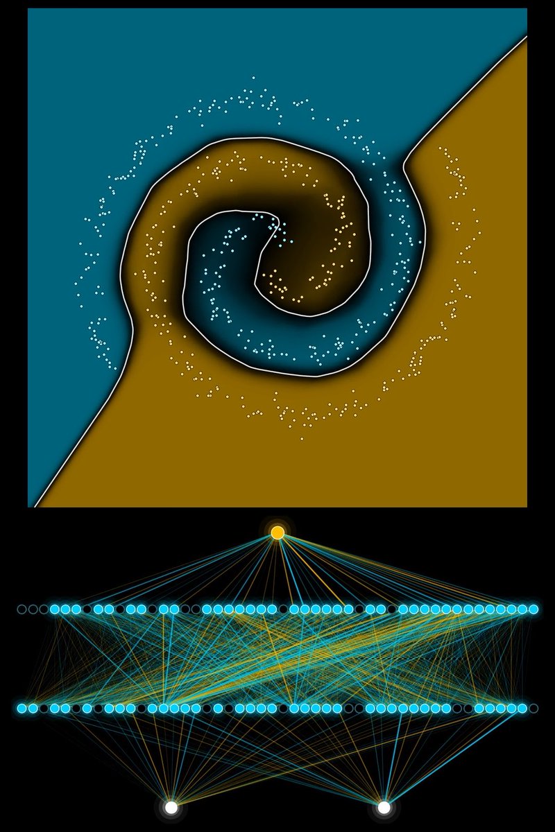
➡️ Machine Learning from Scratch, part 48: the Boltzmann machine. In 1985 Hinton, David Ackley and Terrence Sejnowski published how a Boltzmann machine learns, starting from the Hopfield network of part 47. Like the Hopfield network it prefers pictures with low energy, but it also has hidden units next...

14,700 просмотров • 13 дней назад •via TikTok

Комментарии: 0

Нет доступных комментариев

Здесь появятся комментарии из оригинального поста

Похожие видео

➡️ Machine Learning from Scratch, part 47: the Hopfield network. In 1982 the physicist John Hopfield described a network that works as a memory, and 42 years later this work was part of the Nobel Prize in Physics. Each neuron is one pixel that is either on or off, and every neuron is connected to every other neuron, so 100 pixels need 4,950 connections. There are no layers: signals go back and forth until the network settles. Each neuron takes a weighted sum of its inputs and switches on if the sum is positive, off if it is negative. Storing a picture is simple: for every pair of pixels with the same colour the connection gets stronger, otherwise weaker. Every stored picture becomes a valley in the energy landscape, and no switch can ever raise the energy, so a noisy picture rolls downhill into the nearest stored memory. The code (hopfield.py, 16 lines of numpy, pictures in pics.txt) stores three 10 x 10 pictures, a heart, a house and a smiley, and flips 30 of the 100 pixels in each. After a single pass over all neurons all three come back exactly; the energy of the heart falls from -6.90 to -48.90, the energy of the stored heart. With 100 neurons and random patterns (10 flipped pixels, 20 runs) it recalls 5 patterns every time, 10 patterns in 94.5 % of the cases, 14 in 68 %, 20 in about one in four (24 %) and 30 in 1 %. Honest notes: the weights are kept as whole numbers (100 times the Hebb weight), so a sum of exactly zero switches the neuron on, as the rule says. The landscape in the video is a picture of the idea; the valley floors and the height of the rolling ball are the real energies from the run. #machinelearning #ai #coding #neuralnetworks #nobelprize

MachineLearningToGo

12,000 просмотров • 14 дней назад

➡️ Machine Learning from Scratch, part 15: a recommender, the kind of algorithm that picks what your feed shows you. Our app is simulated: 300 people and 60 videos. Every person has a hidden taste, every video has a hidden style, and each person has watched only about 12 of the 60 videos. All the algorithm ever sees is who liked which of the videos they watched. How it learns: every person gets two numbers, and every video gets two numbers. Think of them as arrows on a map. For every video a person has seen, the two arrows turn into a chance of a like with the sigmoid from part 2. The algorithm compares that chance with what really happened and nudges both arrows a little. That is gradient descent from part 8, and the whole method is called matrix factorisation. The results, all measured on the videos nobody showed it: After 25 rounds it guesses 85.0% of the hidden likes right. After 3000 rounds it gets 87.8% right. The best any method could do here is 91.1%, because some likes are just random. For every person it recommends the three unseen videos with the strongest match, and 98% of them are videos the person really likes. A random unseen video gets a like 51% of the time. The first person on the list watched only 5 videos. From those five it guessed the other 55 and got 51 of them right. We ran the same program on 20 different simulated apps, and it always landed between 84 and 88%. Real apps use hundreds of numbers for every person and every video, plus signals like watch time and skips. The core idea stays the same: learn numbers for people and for videos, and match them. #machinelearning #ai #recommendersystem #python #coding

MachineLearningToGo

88,400 просмотров • 1 месяц назад

➡️ Machine Learning from Scratch, part 31: the transformer. A transformer turns every token into a list of numbers, adds its position, and then lets every token look at the others. That step is called attention: each token has a query (what am I looking for), a key (what do I contain) and a value (what I pass on). The better a query matches a key, the more of that value flows in. Real transformers repeat this in many layers with several attention heads each. The design comes from the 2017 Google paper "Attention Is All You Need" by Ashish Vaswani and colleagues, first used for translation. A large language model is a transformer trained to predict the next token, again and again, on a huge amount of text. Our own run, nothing downloaded. attention.py is one self-attention layer in 16 lines of numpy. Every word gets a query, a key and a value of 8 numbers, starting random, trained from scratch with hand-written backpropagation on 192 made-up sentences like "the dog ate the carrot because it was hungry". The task: find out which pet "it" means. On 64 new test sentences "it" puts 99.95 percent of its attention on the right word on average (the lowest single sentence gets 99.9 percent; the program prints this as 100%). Before training it was 10 percent, spread evenly. The cat sentence from the video is one of the test sentences. Honest notes: our task is easy on purpose. Every sentence has exactly one pet, so "it" only has to learn to look for pets, and it learns that within the first pass. Real sentences with two candidates need more context, which is what many layers are for. Our small version has no positions, no scaling, no mask, one head, and only "it" asks a question. Every word of the test sentences also appears in training; the combinations are new. The 3D space in the video shows the real keys of our model, projected to three axes (two of them stretched so you can see them). The stacked layers are a sketch. #machinelearning #ai #transformer #python #llm

MachineLearningToGo

80,100 просмотров • 1 месяц назад

if you're struggling on where to start learning ML, here’s a playlist of 30 youtube videos to learn machine learning fundamentals from scratch "Machine Learning: Teach by Doing" is a solid choice to learn both theory and code. (1) Introduction to Machine Learning Teach by Doing: (2) What is Machine Learning? History of Machine Learning: (3) Types of ML Models: (4) 6 steps of any ML project: (5) Install Python and VSCode and run your first code: (6) Linear Classifiers Part 1: (7) Linear Classifiers Part 2: (8) Jupyter Notebook, Numpy and Scikit-Learn: (9) Running the Random Linear Classifier Algorithm in Python: (10) The oldest ML model - Perceptron: (11) Coding the Perceptron: (12) Perceptron Convergence Theorem: (13) Magic of features in Machine Learning: (14) One hot encoding: (15) Logistic Regression Part 1: (16) Cross Entropy Loss: (17) How gradient descent works: (18) Logistic Regression from scratch in Python: (19) Introduction to Regularization: (20) Implementing Regularization in Python: (21) Linear Regression Introduction: (22) Ordinary Least Squares step by step implementation: (23) Ridge regression fundamentals and intuition: (24) Regression recap for interviews: (25) Neural network architecture in 30 minutes: (26) Backpropagation intuition: (27) Neural network activation functions: (28) Momentum in gradient descent: (29) Hands on neural network training in Python: (30) Introduction to Convolutional Neural Networks (CNNs):

ℏεsam

109,764 просмотров • 1 год назад

a playlist of 30 youtube videos to learn machine learning fundamentals from scratch if you're struggling on where to start learning ML, this list goes this "Machine Learning: Teach by Doing" is a solid choice to learn both theory and code. (1) Introduction to Machine Learning Teach by Doing: (2) What is Machine Learning? History of Machine Learning: (3) Types of ML Models: (4) 6 steps of any ML project: (5) Install Python and VSCode and run your first code: (6) Linear Classifiers Part 1: (7) Linear Classifiers Part 2: (8) Jupyter Notebook, Numpy and Scikit-Learn: (9) Running the Random Linear Classifier Algorithm in Python: (10) The oldest ML model - Perceptron: (11) Coding the Perceptron: (12) Perceptron Convergence Theorem: (13) Magic of features in Machine Learning: (14) One hot encoding: (15) Logistic Regression Part 1: (16) Cross Entropy Loss: (17) How gradient descent works: (18) Logistic Regression from scratch in Python: (19) Introduction to Regularization: (20) Implementing Regularization in Python: (21) Linear Regression Introduction: (22) Ordinary Least Squares step by step implementation: (23) Ridge regression fundamentals and intuition: (24) Regression recap for interviews: (25) Neural network architecture in 30 minutes: (26) Backpropagation intuition: (27) Neural network activation functions: (28) Momentum in gradient descent: (29) Hands on neural network training in Python: (30) Introduction to Convolutional Neural Networks (CNNs):

ℏεsam

117,748 просмотров • 1 год назад

➡️ Part 9 of learning ML code from scratch Six weights, one wrong answer, and not one of them knows it was at fault. Backpropagation is how they find out. Two questions guide the video: what even is backpropagation, and why do models need it? Step 1, the forward pass. Two numbers go into a tiny network, run through a hidden layer, and one number comes out. Ours says 0.700. We wanted 1.0, so square the difference and the loss is 0.09. That single number is how wrong the model is. Step 2, the question. Six weights produced that answer together. Which of them is to blame, and by how much? Step 3, the one idea. Change a single weight by a tiny amount and watch the error move. How much the error changes per unit of weight is the gradient of that weight. In the video you can see it happen: the weight wobbles and the error bar answers. Step 4, the shortcut. Every weight running into the same neuron starts from one shared number, the blame of that neuron. Multiply that blame by the value each weight carried and you have its gradient. One blame, computed once, and every weight into that neuron gets its own gradient from it. That is why backpropagation is fast enough to train anything at all. Step 5, backwards. The blame starts at the output and every layer hands its share to the layer in front of it, back through the same network the data came forward through. It goes layer by layer, and inside one layer every neuron is done together. Step 6, the update. The optimizer moves every weight against its own gradient, the whole weight matrix in one go, so no weight waits for its turn. All six gradients here are negative, so all six weights go up. After one step the answer reads 0.769. After sixty it reads 0.968 and the error is down to 0.001. The honest part: every gradient in the video was checked against the measured change of the error. Move that one weight, see what the error does, divide. Backprop and the measurement agree to nine decimal places, otherwise nothing would have rendered. #machinelearning #backpropagation #neuralnetworks #python #coding

MachineLearningToGo

210,600 просмотров • 1 месяц назад