Loading video...

Video Failed to Load

Go Home

The vacuum is not always stable Using the nonlinear Klein-Gordon equation, bubbles of a lower-energy state erupt across the fabric expand, collide and leave oscillating remnant behind called Oscillons.

10,768 views • 11 days ago •via X (Twitter)

13 Comments

Rozmowy z Bogiem's profile picture
Rozmowy z Bogiem11 days ago

Where does the cause lie?

andy's profile picture
andy11 days ago

another banger

Brian Jordan's profile picture
Brian Jordan11 days ago

Next level, keep exploring!!

Edwin VanGorder's profile picture
Edwin VanGorder11 days ago

the curve to corners modells the heptagon saddleback geometry to hyperbolic plane linking split octonions cosmogenesis on numberline to spectral grading through the pseudo algebras...where an apeirogon models inversion to Holographic horizon transport

Monsol's profile picture
Monsol10 days ago

It's hard to visualize this as 3d model bubbles inside bubbles affecting other bubbles.

Carlos ‘Cacho’ Contreras's profile picture
Carlos ‘Cacho’ Contreras11 days ago

What song is that?

Carlos ‘Cacho’ Contreras's profile picture
Carlos ‘Cacho’ Contreras11 days ago

OMG, that's so nice of you, thank you so much! 🫶

Mathelirium's profile picture
Mathelirium11 days ago

Youre welcome! Im using a cleaner version from AppleMusic but I forgot the name of the song. Mayne you can if you know some Arabic

Carlos ‘Cacho’ Contreras's profile picture
Carlos ‘Cacho’ Contreras11 days ago

I don't know any Arabic, but I'll find it, BELIEVE ME! Love it.

Heather Davis's profile picture
Heather Davis11 days ago

Cymatics

V. W.'s profile picture
V. W.11 days ago

In what sense, then, is anything truly stable?

ArtisanTony's profile picture
ArtisanTony11 days ago

But the vacuum does don’t have edges to bounce off of ;)

PoetinAz's profile picture
PoetinAz11 days ago

You mean your vacuum oscillates like an old fan in your grandma’s house?? Wow that is awesome!!

Related Videos

Quantum Mechanics Series Lecture 4 Lecture 1 established that ρ(x,t) = |ψ(x,t)|² behaves like a conserved probability density. Lecture 2 showed what drives that flow. We also saw that writing ψ = r exp(iθ) makes the probability current proportional to the phase gradient, making it clear that phase geometry literally steers the motion. Lecture 3 then showed that the centroid of that flow can move almost classically when the packet is tight and the external potential is smooth. However, that raises yet another question. If the centroid can look classical, why does the full wave still spread, bend, split, and interfere in ways no classical particle cloud would? This is because the wave is not driven only by the external potential. It is also driven by its own curvature. Write ψ(x,t) = r(x,t) exp(iθ(x,t)) with ρ = r². Then Schrödinger’s equation gives two coupled real equations. One is the continuity equation you already know. The other looks like a Hamilton-Jacobi equation, but with one extra term: Q = −(1/2m) ∇²r / r This is the so-called Quantum Potential. It depends entirely on how the amplitude bends across space. So, the wave is being shaped not only by V(x,t), but also by the geometry of its own envelope. In the animation, the upper surface is still |ψ| and its skin is still colored by arg(ψ). The glowing threads still trace the probability current. But now a second membrane hangs underneath. That lower membrane encodes the quantum potential Q itself. The porcelain bead marks the quantum centroid. The amber bead follows a classical centroid under the same external V. When those paths separate, the lower membrane tells you why. The difference is not magic but the extra term classical mechanics does not have. The math breakdown: Start from Schrödinger evolution in units with ħ = 1: i ∂ψ/∂t = [ −(1/2m) ∇² + V(x,t) ] ψ Write the state in polar form: ψ = r exp(iθ) Then ρ = |ψ|² = r² From the imaginary part, you recover probability conservation: ∂ρ/∂t + ∇·j = 0 with j = (1/m) Im(ψ* ∇ψ) = (ρ/m) ∇θ So the local velocity field is v = j / ρ = ∇θ / m Now take the real part of Schrödinger’s equation. That gives ∂θ/∂t + |∇θ|² / (2m) + V + Q = 0 where Q = −(1/2m) ∇²r / r This is the classical Hamilton-Jacobi equation with one extra term. That extra term is what makes quantum motion locally different from classical motion. Take a gradient of that phase equation and use v = ∇θ / m. Then the flow obeys an Euler-like equation: ∂v/∂t + (v·∇)v = −(1/m) ∇(V + Q) In other words, there are really two forces in the problem. One comes from the external potential V. The other comes from the wave’s own curvature through Q. That is why Ehrenfest is only approximate. The centroid can still satisfy d⟨x⟩/dt = ⟨p⟩/m d⟨p⟩/dt = −⟨∇V⟩ but the internal shape of the packet evolves under the combined influence of V and Q. When the packet stays broad and smooth, Q is gentle and the motion looks more classical. When the packet develops sharp curvature or interference structure, Q becomes strong and the classical picture breaks down. That is what this scene is designed to show live. #QuantumMechanics #Wavefunction #SchrodingerEquation #BornRule #ProbabilityCurrent #ContinuityEquation #Phase #EhrenfestTheorem #QuantumPotential #Madelung #HamiltonJacobi #MathematicalPhysics #Mathematics #Physics

Mathelirium

20,653 views • 6 months ago

Lecture 2 on our Quantum Mechanics Series Schrödinger’s equation doesn’t start from mystery. It starts from a very specific bet…the state of a particle is a complex field ψ(x,t), and whatever dynamics we write down must move ψ forward in time in a way that preserves total probability. We ask a basic question…what equation should ψ satisfy so that |ψ|² behaves like a conserved density, the way mass density does in fluid flow? What is ψ? Think of ψ(x,t) as the amplitude assigned to “the particle is at position x at time t”. It’s not a probability. It’s the object you add first, and only at the end do you square p(x,t) = |ψ(x,t)|² Because ψ is complex, it has magnitude and phase. Write it in polar form ψ(x,t) = r(x,t) exp(i θ(x,t)) Then r² = |ψ|² is the density, and θ will end up controlling flow (the probability current). Where does Schrödinger’s equation come from? Start with two empirical inputs about waves and particles: E = ħ ω p = ħ k Here ħ (“h-bar”) is Planck’s constant divided by 2π. It’s the unit conversion factor between the wave description (frequency ω, wavevector k) and the particle description (energy E, momentum p). In units, ħ has units of joule-seconds, so multiplying ω (1/seconds) gives energy (joules), and multiplying k (1/meters) gives momentum (kg·m/s). It’s the number that tells you how much energy or momentum you get per unit frequency or wavenumber. A plane wave with angular frequency ω and wavevector k is ψ(x,t) = A exp(i(k·x − ω t)) Now notice what derivatives do to this wave: ∂ψ/∂t = −i ω ψ ∇ψ = i k ψ ∇²ψ = −|k|² ψ Multiply those identities by ħ: i ħ ∂ψ/∂t = ħ ω ψ = E ψ −i ħ ∇ψ = ħ k ψ = p ψ −ħ² ∇²ψ = ħ² |k|² ψ = p² ψ So for plane waves, the operators Ê = i ħ ∂/∂t p̂ = −i ħ ∇ act like energy and momentum! Now use the classical nonrelativistic energy relation: E = p²/(2m) + V(x) This is bookkeeping for a particle moving slow enough that relativity can be ignored. The term p²/(2m) is kinetic energy. If p = mv, then p²/(2m) = (m²v²)/(2m) = (1/2)mv². The term V(x) is potential energy. It depends on position because forces come from spatially varying energy. A slope in V pushes the particle. Examples: for a charged particle in an electric potential φ(x), V(x) = q φ(x). Near Earth, V(z) = mgz. The point is total energy equals kinetic plus potential. Turn that into an equation for ψ by replacing E and p with the operators above: Ê ψ = (p̂²/(2m) + V) ψ Compute p̂² = (−i ħ ∇)·(−i ħ ∇) = −ħ² ∇², so we get i ħ ∂ψ/∂t = ( −ħ²/(2m) ∇² + V(x) ) ψ That is the time-dependent Schrödinger equation. The derivation here is a controlled heuristic: we matched the plane-wave identities to the measured relations E = ħω and p = ħk, then imposed the same energy bookkeeping as classical mechanics. Why this equation is the right kind of rule If ψ is the state, we need a rule that preserves total probability: ∫ |ψ(x,t)|² dx = 1 Schrödinger evolution does. You can see it by deriving a continuity equation. Let ρ(x,t) = |ψ|² = ψ* ψ. Take a time derivative: ∂ρ/∂t = ψ* ∂ψ/∂t + ψ ∂ψ*/∂t Use Schrödinger and its complex conjugate: ∂ψ/∂t = (1/(i ħ)) ( −ħ²/(2m) ∇²ψ + Vψ ) ∂ψ*/∂t = (−1/(i ħ)) ( −ħ²/(2m) ∇²ψ* + Vψ* ) Plug in. The V terms cancel exactly, and what remains can be rearranged into a divergence: ∂ρ/∂t + ∇·j = 0 where the probability current is j = (ħ/(2mi)) ( ψ* ∇ψ − ψ ∇ψ* ) This is the best way to explain ehat ψ is: |ψ|² behaves like a conserved density, and the phase of ψ is what drives the current j. So in this series, ψ isn’t a slogan. It’s the object whose modulus squared is the density, whose phase generates flow, and whose time evolution is fixed (up to V) by matching wave relations to energy bookkeeping: i ħ ∂ψ/∂t = ( -ħ²/(2m) ∇² + V ) ψ #QuantumMechanics #SchrodingerEquation #WaveFunction #BornRule #Physics #MathematicalPhysics

Mathelirium

40,978 views • 9 months ago

Final Lecture of our Statistical Mechanics Series. Lecture 2 showed how we move from the Full Phase-Space Density ρ(q₁, …, qₙ, p₁, …, pₙ, t) to smaller statistical objects by integrating out variables we do not want to keep. That gives reduced descriptions like the One-Particle Density f₁(q₁,p₁,t) and the Two-Particle Density f₂(q₁,p₁,q₂,p₂,t) This was the simplification. Now comes the catch. If the Full Density obeys Liouville’s Equation, the reduced densities do not evolve independently. The equation for one level depends on the next one and this is referred to as the BBGKY hierarchy. The One-Particle Density depends on the Two-Particle Density. The Two-Particle Density depends on the Three-Particle Density. And the chain keeps going. That happens because particles interact. Once one particle feels the rest, one-particle information is no longer enough. Correlations enter, and the lower level is fed from above. If the full Hamiltonian is H = Σᵢ pᵢ²/(2m) + Σᵢ U(qᵢ) + (1/2) Σᵢ Σⱼ≠ᵢ Φ(qᵢ − qⱼ) then reducing the full density does not make the interaction terms disappear. It leaves behind coupling to higher-order reduced densities. So, schematically, ∂f₁/∂t + transport of one particle = interaction term involving f₂ and more generally the heirarchy is such that ∂fₛ/∂t + s-particle transport = interaction term involving fₛ₊₁ Therefore, Lecture 3 is really about the price of reduction. We simplify the description, but the information we remove comes back as coupling to higher-order correlations. So, how do you actually compute anything if every level depends on the next one? This is the so-called Closure Problem. To make the hierarchy usable, you need an extra assumption that cuts the chain. You replace the exact higher-order object by an approximation in terms of lower-order ones. The most basic example is a factorized closure at the pair level, where the exact correlated Two-Particle Density is replaced schematically by a product of One-Particle Densities: f₂(q₁,p₁,q₂,p₂,t) ≈ f₁(q₁,p₁,t) f₁(q₂,p₂,t) That approximation is not exact. It throws away part of the correlation structure. But it gives you something the raw hierarchy does not... a closed equation for the lower-level description. That is why closure matters so much. Without it, the hierarchy is exact but open. With it, the theory becomes approximate but usable. Thus, the combined point of this final Statistical Mechanics post is simple. First, reduced descriptions are not closed because interactions generate correlations across levels. Second, if you want a workable Kinetic Theory, you must close the hierarchy by approximating those higher-order correlations. It is the bridge from formal many-body mechanics to equations people can actually solve. In the render, that is exactly the story you are seeing. The first part shows the hierarchy itself: one reduced level feeding the next, with lower descriptions inheriting structure from higher ones. The second part shows the closure step where the exact correlated pair level is replaced by a factorized ansatz, and that approximation gives back a closed one-particle description. That is, the animation moves from dependence to approximation, and from approximation to solvability. #StatisticalMechanics #BBGKY #ClosureProblem #KineticTheory #PhaseSpace #ReducedDistribution #HamiltonianMechanics #MathematicalPhysics #Mathematics #Physics

Mathelirium

10,998 views • 5 months ago

The Mathematics of Moving a Cursor with Neural Signals What might Neuralink Neuralink be doing Mathematically? Consider the task of moving a cursor without touching it. The machine is not looking for a full thought, a sentence, or an image. For this Control problem, the useful object is an intended movement state. sₜ = (pₜ, vₜ) Here, pₜ is the cursor position at time t, and vₜ is the velocity the user is trying to express. The implant records neural activity through many electrode channels, then the decoder tries to estimate vₜ from that activity. Neuralink’s PRIME material describes the N1 Implant as recording and transmitting brain activity with the goal of enabling computer control. For channel i, a simple population model is rᵢ(t) ≈ bᵢ + aᵢ max(0, dᵢ · vₜ) + ηᵢ(t) where rᵢ(t) is the measured activity, bᵢ is baseline activity, aᵢ is channel gain, dᵢ is the channel’s preferred movement direction, and ηᵢ(t) is noise. One channel is not the command. The useful signal is the pattern across many channels: rₜ = (r₁(t), r₂(t), …, rₙ(t)) The decoder subtracts the baseline vector b and applies a learned map W: v̂ₜ = W(rₜ − b) This gives an estimate of the intended velocity. The cursor then updates by pₜ₊₁ = pₜ + Δt v̂ₜ This is the loop shown in the render: neural activity -> decoded velocity -> cursor motion The cortical network and electrode threads show the measurement side. The N1 Implant is described as using 1,024 electrodes distributed across 64 flexible threads, each thinner than a human hair. The decoder panel shows the computational side with activity rₜ, decoded velocity v̂ₜ, and the cursor state pₜ changing over time. A noisy biological pattern becomes a state estimate. That estimate becomes motion on a screen. Therefore, the first lesson is not that Neuralink makes the brain a screen. For cursor control, the Mathematics is more precise: A small piece of intention is represented as a hidden state, measured through neural activity, decoded as a vector, and turned into action. #Neuralink #BrainComputerInterface #NeuralEngineering #Mathematics #StateEstimation #Neuroscience #MachineLearning #BiomedicalEngineering

Mathelirium

14,520 views • 5 months ago