Microsoft made 100B parameter models run on a single... CPU. bitnet.cpp: The official inference framework for 1-bit LLMs. The math behind 1-bit LLMs is what makes them revolutionary. Traditional LLMs use 16-bit floating point weights. Every parameter is a number like 0.0023847 or -1.4729. When you run inference, you multiply these floats together. Billions of times. That's why you need GPUs, they're optimized for floating point matrix multiplication. BitNet b1.58 uses ternary weights: {-1, 0, 1}. That's not a simplification. That's a fundamental change in the math. When your weights are only -1, 0, or 1: → Multiply by 1 = keep the value → Multiply by -1 = flip the sign → Multiply by 0 = skip entirely Matrix multiplication becomes addition and subtraction. No floating point operations. No GPU required. This is why bitnet.cpp achieves: → 2.37x to 6.17x speedup on x86 CPUs → 1.37x to 5.07x speedup on ARM CPUs → 71.9% to 82.2% energy reduction on x86 → 55.4% to 70.0% energy reduction on ARM The speedups scale with model size. Larger models see bigger gains because there are more operations to simplify. A 100B parameter model running at human reading speed (5-7 tokens/second) on a single CPU. That's not optimization. That's a different paradigm. Why 1.58 bits? Because log₂(3) ≈ 1.58. Three possible values = 1.58 bits of information per weight. The key insight: These models aren't quantized after training. They're trained from scratch with ternary weights. The model learns to work within the constraint. No precision loss. No quality tradeoff.show more

[VAE] by Hand ✍️ A Variational Auto Encoder (VAE)... learns the structure (mean and variance) of hidden features and generates new data from the learned structure. In contrast, GANs only learn to generate new data to fool a discriminator; they may not necessarily know the underlying structure of the data. The International Conference on Learning Representations (ICLR) this year announced its first ever "Test of Time Award" to recognizes the VAE paper, published 10 years ago. This exercise demonstrates how to calculate a VAE by hand. [1] Given: ↳ Three training examples X1, X2, X3 ↳ Copy training examples to the bottom ↳ The purpose is to train the network to reconstruct the training examples. ↳ Since each target is a training example itself, we use the Greek word "auto" which means "self." This crucial step is what makes an autoencoder "auto." [2] Encoder: Layer 1 + ReLU ↳ Multiply inputs with weights and biases ↳ Apply ReLU, crossing out negative values (-1 -> 0) [3] Encoder: Mean and Variance ↳ Multiply features with two sets of weights and biases ↳ 🟩 The first set predicts the means (𝜇) of latent distributions ↳ 🟪 The second set predicts the standard deviation (𝜎) of latent distributions [4] Reparameterization Trick: Random Offset ↳ Sample epsilon ε from the normal distribution with mean = 0 and variance = 1. ↳ The purpose is to randomly pick a offset away from the mean. ↳ Multiply the standard deviation values with epsilon values. ↳ The purpose is to scale the offset by the standard deviation. [5] Reparameterization Trick: Mean + Offset ↳ Add the sampled offset to predicted mean ↳ The result are new parameters or features 🟨 as inputs to the Decoder. [6] Decoder: Layer 1 + ReLU ↳ Multiply input features with weights and biases ↳ Apply ReLU, crossing out negative values. Here, -4 is crossed out. [7] Decoder: Layer 2 ↳ Multiply features with weights and biases ↳ The output is Decoder's attempt to reconstruct the input data X from reparameterized distributions described by 𝜇 and 𝜎. [8]-[10] KL Divergence Loss [8] Loss Gradient: Mean 𝜇 ↳ We want 𝜇 to approach 0. ↳ A lot of math called SGVB simplifies the calculation of loss gradients to simply 𝜇 [9,10] Loss Gradient: Stdev 𝜎 ↳ We want 𝜎 to approach 1. ↳ A lot of math simplifies the calculation to 𝜎 - (1/ 𝜎) [11] Reconstruction Loss ↳ We want the reconstructed data Y (dark 🟧) to be the same as the input data X. ↳ Some math involving Mean Square Error simplifies the calculation to Y - X.show more

[Backpropagation] by Hand✍️ [1] Forward Pass ↳ Given a... multi layer perceptron (3 levels), an input vector X, predictions Y^{Pred} = [0.5, 0.5, 0], and ground truth label Y^{Target} = [0, 1, 0]. [2] Backpropagation ↳ Insert cells to hold our calculations. [3] Layer 3 - Softmax (blue) ↳ Calculate ∂L / ∂z3 directly using the simple equation: Y^{Pred} - Y^{Target} = [0.5, -0.5, 0]. ↳ This simple equation is the benefit of using Softmax and Cross Entropy Loss together. [4] Layer 3 - Weights (orange) & Biases (black) ↳ Calculate ∂L / ∂W3 and ∂L / ∂b3 by multiplying ∂L / ∂z3 and [ a2 | 1 ]. [5] Layer 2 - Activations (green) ↳ Calculate ∂L / ∂a2 by multiplying ∂L / ∂z3 and W3. [6] Layer 2 - ReLU (blue) ↳ Calculate ∂L / ∂z2 by multiplying ∂L / ∂a2 with 1 for positive values and 0 otherwise. [7] Layer 2 - Weights (orange) & Biases (black) ↳ Calculate ∂L / ∂W2 and ∂L / ∂b2 by multiplying ∂L / ∂z2 and [ a1 | 1 ]. [8] Layer 1 - Activations (green) ↳ Calculate ∂L / ∂a1 by multiplying ∂L / ∂z2 and W2. [9] Layer 1 - ReLU (blue) ↳ Calculate ∂L / ∂z1 by multiplying ∂L / ∂a1 with 1 for positive values and 0 otherwise. [10] Layer 1 - Weights (orange) & Biases (black) ↳ Calculate ∂L / ∂W1 and ∂L / ∂b1 by multiplying ∂L / ∂z1 and [ x | 1 ]. [11] Gradient Descent ↳ Update weights and biases (typically a learning rate is applied here). 💡 Matrix Multiplication is All You Need: Just like in the forward pass, backpropagation is all about matrix multiplications. You can definitely do everything by hand as I demonstrated in this exercise, albeit slow and imperfect. This is why GPU's ability to multiply matrices efficiently plays such an important role in the deep learning evolution. This is why NVIDIA is now close to $1 trillion in valuation. 💡Exploding Gradients: We can already see the gradients are getting larger as we back-propagate up, even in this simple 3-layer network. This motivates using methods like skip connections to handle exploding (or diminishing) gradients as in the ResNet. I did the calculations entirely by hand. Please let me know if you spot any error or have any questions!show more

[Discrete Fourier Transform] by Hand ✍️ In signal processing,... the Discrete Fourier Transform (DFT) is no doubt the most important method. But the math involved is extremely complex, literally, involving a summation over a complex number term e^(-iwt). I developed this exercise to demonstrate that underneath such complexity, DFT is just a series of matrix multiplications you can calculate by hand. ✍️ Once you see that, it should not surprise you that a deep neural network, which is also a series of matrix multiplications, with activation functions in-between, can learn to perform DFT to process and analyze signals so effectively. How does DFT work? [1] Given ↳ Signals A, B, and C in the 🟧 frequency domain: ◦ A = cos(w) + 2cos(2w) ◦ B = cos(w) + cos(3w) + cos(4w) ◦ C = -cos(2w) + cos(3w) ◦ Each signal is a weighed sum of four cosine waves at frequencies 1w, 2w, 3w, and 4w. ◦ We will apply Inverse DFT to convert the signals to time domain representations, and then demonstrate DFT can convert back to their original frequency domain representations. ↳ Signal X in the 🟩 time domain. X is sampled at 10 time points 1t, 2t, …, 10t: ◦ X = [-2.5, -1.8, 3, -0.7, -1.0, -0.7, 3, -1.8, -2.5, 5] ◦ Suppose X is also a weighted sum of the same four cosine waves, but we don’t already know their weights. We will apply DFT to discover them. [2] 🟧 Frequency Matrix (F) ↳ Write the coefficients of A, B, C as a matrix F. Each signal is a row. Each frequency is a column. ↳ A → [1, 2, 0, 0] ↳ B → [1, 0, 1, 1] ↳ C → [0, 1-, 1, 0] [3] Cosine → Discrete ↳ Sample from the continuous cosine waves at discrete time points 1t, 2t, 3t, to 10t. [4] Cosine Matrix (W) ↳ Write the samples as a matrix, Each frequency is a row. Each time point is a column. [5] Inverse DFT: 🟧 Frequency → 🟩 Time ↳ Multiply the frequency matrix F and the cosine matrix W. ↳ The meaning of this multiplication is to linearly combine the four cosine waves (rows in W) into time-domain signals (rows in T) using the weights specified in F. ↳ The result is matrix T, which are signals A, B, C converted to the time domain. Each signal is a row. Each time point is a column. [6] Transpose ↳ Transpose T, converting each signal’s time domain representation from a row to a column. [7] DFT: 🟩 Time → 🟧 Frequency ↳ Multiply the cosine matrix W with the transpose of matrix T. ↳ The purpose of this multiplication is to take a dot-product between each time-domain signal (columns in the transpose of T) and each cosine wave (rows in W), which has the effect of projecting the signal onto a cosine wave to determine how much they are correlated. Zero means not correlated at all. ↳ The result is an intermediate version of the “recovered” frequency matrix where each column corresponds to a signal and each row corresponds to a frequency. ↳ Compared to the original frequency matrix F, this intermediate matrix has non-zero weights in the correct places, but scaled up by a factor of 5 (n/2, n=10). For example, signal A, originally [1,2,0,0], is recovered at [5,10,0,0]. [8] Scale ↳ Multiply each value by 2/n = 1/5 to scale down the intermediate matrix to match the magnitude of the original frequency matrix F. [9] Transpose ↳ Transpose the recovered frequency matrix back to the same orientation of the original frequency matrix F. ↳ Like magic 🪄, the result is identical to the original F, which means DFT successfully recovered the frequency components of signals A, B, C. [10] Apply DFT to X: 🟩 Time → 🟧 Frequency ↳ Now that we have some confidence in DFT’s ability to recover frequency components, we apply DFT to X’s time-domain representation by multiplying W with X. ↳ The result is the an intermediate matrix. [11] Scale ↳ Similarly, we scale down by a factor of 5 to obtain the recovered frequency components of X (a column). [12] Transpose ↳ Similarly, we transpose the recovered column to row to match the orientation of the frequency matrix. ↳ Using the coefficients [0,0,3,2], we can write the equation of X as 3cos(3w) + 2cos(4w). Notes: I hope this by hand exercise helps you understand the essence of DFT. But there is more technical details, such as: • Sine: The complete DFT math also includes sine waves that follow a similar calculation process. • Phase: Here, we assume all the cosine waves are aligned at the origin, namely, phase is 0. If a phase p is added, for example, cos(w+p), we will need to calculate the sine component and use their ratio to figure out what p is. • Magnitude: If phase is not zero, the magnitude will need to be calculated by combining both cosine and sine terms.show more

90% of "AI developers" just download pre packaged GGUF... files from Hugging Face, hit run, and call it a day. The top 10% know how to pull the raw safetensors, run the math, and quantize massive models into Q4_K_M themselves. If you think llama.cpp can only execute models, you’re missing the best part of the open source ecosystem. It’s a high performance optimization suite. Manually stripping 69% of the VRAM footprint off a brand new model architecture is where real infrastructure value is made. If you want to actually master local inference and deploy models like Google’s massive Gemma 4 12B it on consumer NVIDIA hardware using llama.cpp, you need to learn this pipeline. Let's build it. I just took the raw 22.7 GB Gemma 4 baseline and manually compressed it down to a 7.02 GB Q4_K_M GGUF artifact using llama.cpp. That is a 69% reduction in footprint. No quality loss. No VRAM bottlenecks. Just native, hardware accelerated C++ inference running a full 2,50,000 token context window on a dual NVIDIA Tesla T4 setup. Stop melting your VRAM on unoptimized weights and stop relying on other people's pipelines. Own your stack. I mapped this entire architecture from dynamic binary fetching to raw quantization and real time GPU streaming into a single, bulletproof notebook. Notebook link is in the comments below. Bookmark this blueprint for your next deployment and tell me which quantization works best for your workflow and model.show more

look what a single consumer GPU just built. gave... Qwen3.5-35B-A3B one prompt: build a cloud GPU marketplace with pricing cards, deploy templates, and a benchmark leaderboard. it planned the layout, wrote the animations, populated the data, and served it. one shot. one HTML file. then i told it to iterate. split the hero, add a floating GPU with neural network animation. glassmorphism on the cards. done. done. done. three rounds, no confusion, no regressions. 4-bit quantized. 19.7 GB. single RTX 3090. full coding agent claude code harness running on localhost. no API calls leaving my machine. no subscription. no rate limits. earlier today i pointed it at my own production website. it curled the HTML, found every broken link, and told me "pretty shell, empty core. would not recommend." then built a better version from scratch. local inference stops being a demo when you actually steer it. the models are there. they understand intent. but you have to meet them halfway with good prompts, clear context, and real project structure. that's the skill gap now. not the models. the steering. more experiments coming. i genuinely cannot stop playing with this thing.show more

Run Gemma 4 26B MoE on 8GB VRAM with... 250k context at 20+ tokens/sec If you own any 8GB VRAM graphics card, stop what you are doing. Local AI just had its absolute "Holy Shit" moment for budget hardware. Yesterday, I benchmarked Unsloth Gemma 4 12B Q4_K_XL on an 8GB card. The community went wild but immediately demanded more: "Can we run a 25B+ model on budget GPUs?" Today, I’m delivering exactly that. I am running a massive 26B parameter Mixture of Experts (MoE) model locally on a standard 8GB VRAM setup with 250k full native context!. If you own an RTX 3060, 3070, 4060, or any budget GPU with 8GB of VRAM, the local AI paradigm has completely changed. The performance metrics are astonishing: - 20 tokens/sec flat decode throughput. - Stable, flat decode speed even with massive prompts. - I threw a 60k token prompt at it, and it still clocked in at 20 TPS without dropping a single frame. # What about prefill? Yes, Time To First Token (TTFT) is slightly high when swallowing massive contexts. But with a solid 200 tokens/sec prefill speed, the wait is barely noticeable and highly usable. And this is running completely without Multi Token Prediction (MTP) active. How is this possible? It’s the magic of Google's new QAT (Quantization Aware Training) quants for Gemma 4. The model weight file (unsloth gemma-4-26B-A4B-it-qat-UD-Q4_K_XL.gguf) is only 13.2 GB, making it the ultimate local powerhouse. # The Test Setup: CPU: Intel Core i7 RAM: 16GB System RAM GPU: NVIDIA GeForce RTX 4060 Laptop GPU (8GB VRAM) # The Secret Sauce (The -cmoe Flag) To make this work properly on any 8GB card, you must use the -cmoe (CPU MoE) flag in llama.cpp. This flag isolates the heavy MoE expert weights directly to system memory (CPU/RAM) while letting your GPU focus strictly on the Attention layers and the KV Cache. It prevents VRAM spillage and holds the throughput rock solid. # The flags: -m "gemma-4-26B-A4B-it-qat-UD-Q4_K_XL.gguf" -cmoe -c 248000 -v Once running, just open the UI on localhost and toggle the new reasoning lightbulb icon in the text input box to watch the model perform multi step thinking. Are you still running smaller models, or are you ready to scale up your budget local setups? Let's discuss in the repliesshow more

we sped up distributed inference by up to 5x... with decentralized speculative decoding. many don't realize that AI models normally generate text one single word at a time, waiting for the network after every word. speculative decoding changes this by using a "guess & confirm" system, similar to autocomplete. how it's done: 1. draft locally (the guess) instead of waiting for the network, a tiny, fast model on your device guesses the next few words instantly, without waiting for the network. 2. confirm remotely (the check) the massive remote model doesn't generate from scratch; it just checks the draft. it looks at the guesses in a batch and says "yes, yes, no." you get multiple words in the time it usually takes to get one. 3. adaptive logic dsd is smart. if the topic is creative, it lets the draft flow loose. if the topic is math or code, it checks more strictly. it balances speed and precision automatically so your inference almost feel instant. find out more: paper: blog:show more

This Chinese developer launched Llama 70B locally on a... MacBook on a plane and for a full 11 hours without internet ran client projects. He was sitting by the window on a transatlantic flight with a MacBook Pro M4 with 64 GB of memory. WiFi on board cost $25 for the flight. He declined. No cloud API, no connection to Anthropic or OpenAI servers, no internet at all. Just a local Llama 3.3 70B on bf16 and his own orchestrator script. The model runs through llama.cpp. Generation speed, 71 tokens per second. Context around 60,000 tokens. Memory usage, 48.6 GiB out of 64. Battery at takeoff, 3 hours 21 minutes. And he gave the orchestrator this system prompt before takeoff: "You are an offline orchestrator running on a single MacBook. There is no network. The only resources you have are local files in /Users/dev/work, the Llama 70B inference server at localhost:8080, and a battery budget of 3 hours 21 minutes. Process the queue at /Users/dev/work/queue.jsonl (one client task per line). For each task: draft → run local evals → save artefact to /Users/dev/work/done/. Save context checkpoints every 12 tasks so you can resume after a battery swap. Stop only on empty queue or when battery drops below 5%." So the system knows exactly what resources it is running on. It knows it has no connection to the outside world for the next 11 hours. It knows it has finite memory and a finite battery. It knows the human will not intervene until the plane lands. The system runs in 1 loop. Takes a task from the queue, runs it through inference, saves the artifact, writes a checkpoint. Task after task, just like that. And only when the battery drops below 5% does the orchestrator automatically pause, waits for the laptop to switch to the backup power bank, and continues from the last checkpoint. Here is what the system actually writes in his log during the flight: "saved context checkpoint 8 of 12 (pos_min = 488, pos_max = 50118, size = 62.813 MiB)" "restored context checkpoint (pos_min = 488, pos_max = 50118)" "prompt processing progress: n_tokens = 50 / 60 818" "task 37016 done | tps = 71 s tokens text → /Users/dev/work/done/proposal_westside.md" Outside the window, clouds, blue sky, and no WiFi. On the tray, 1 MacBook, an open terminal on 2 screens, and an inference server on localhost. From what I have observed, this is the cleanest offline AI workflow I have seen in the past year: 11 hours of flight, $0 for WiFi, and the entire client queue closed before landing.show more

Researchers made KMeans 200x faster. And the new technique... also beats approaches like cuML and FAISS. Flash-KMeans is an IO-aware implementation of exact KMeans that redesigns the algorithm around modern GPU bottlenecks. By attacking the memory bottlenecks directly, Flash-KMeans achieves: - 33x speedup over cuML - 200x speedup over FAISS This speedup comes from how it moves through GPU memory. Standard KMeans runs in two steps, and both are bottlenecked by reads and writes to GPU memory: 1) The first step matches every point to its nearest centroid. Standard KMeans computes the full point-to-centroid distance matrix, writes it out to GPU memory, then reads it back to find each nearest centroid. That write-then-read round trip is the bottleneck. Flash-KMeans combines the distance calculation with the nearest-centroid step, so the result is computed on-chip and the full matrix is never written out. 2) The second step recomputes each centroid by averaging the points assigned to it. Standard KMeans has thousands of threads writing into the same centroid slots at once, so they stall waiting for their turn. Flash-KMeans sorts points by cluster first, turning scattered writes into sequential reductions that read and write memory in one efficient pass. Using these two optimizations at the million-scale, Flash-KMeans completes a standard KMeans iteration in a few milliseconds. The video below depicts this in action. Several reasons why this is important: KMeans has always been an offline primitive. Something you run once to preprocess data and move on. These speedups make the approach viable in several runtime-critical systems. ↳ Vector indices like FAISS use KMeans to build search indices. Faster KMeans means you can re-index dynamically as data changes. ↳ LLM quantization methods need KMeans to find optimal weight codebooks, per layer, repeatedly. What takes hours could now take minutes. ↳ MoE models need fast token routing at inference time. Flash-KMeans makes it viable to run this inside the inference loop, not just in preprocessing. I have shared the paper in the replies. That said, memory is the real constraint Flash-KMeans solves, and the problem is not just limited to clustering. The vectors a RAG system stores after indexing create similar bottlenecks. I wrote a detailed walkthrough recently on cutting this vector memory by 32x with binary quantization, querying 36M+ vectors in a few milliseconds. Read it below.show more

Nvidia just put a $250,000 cloud workload on your... desk for $2,999 - and killed your $1,900/month AWS bill in the process You don't rent it, you don't manage it, you don't pay a single cloud bill - you just plug it in and let it eat the workloads you used to wire to AWS every month It looks like a small Mac mini, it's actually a full GB10 Grace Blackwell stack with 128GB of unified memory running models up to 200B parameters It's called DGX Spark, the consumer version of the rack Nvidia ships to OpenAI The reason Nvidia did this is simple Cloud GPU pricing is a tax on every developer building AI right now $1,900/month per seat, billions in margin flowing to AWS, Lambda, and CoreWeave Nvidia just cut themselves in by removing the cloud entirely Their solution is to skip the middleman, ship the rack to your desk, and let you keep every dollar of margin you used to wire to a hyperscaler This is much cheaper, faster, and you own the asset at the end But there is still a question nobody is answering yet, what happens to AWS, GCP, and Lambda when 500,000 developers move their inference back to a $2,999 box on their desk Also, technically you can stack four of these and run a 1.6 trillion parameter model locally for under $12,000 Even a single Spark out-performs the cloud subscription Anthropic engineers were running two years ago bookmark this, it pays back in 60 days 👇show more

The human brain is truly a marvel of nature.... If you horribly reductive, and boiled it down to a language model, you'd be looking at roughly 100 trillon parameters running as a sparse MoE architecture Only about 1-5% of neurons fire at any given moment, meaning the brain "activates" maybe 1-5 trillion parameters per inference step. For context, the largest AI models we've built probably top out around 5 trillion parameters. The brain is roughly 100x larger. Even its active params at any given moment are larger than almost every model in existence today. Here's what melts my brain (pun intnended) though Your brain does all of this on about 20 watts of power, less than a dim light bulb. Training a frontier AI model consumes enough electricity to power small cities for months. Running inference across data centers pulls megawatts. Your brain runs 24/7 for 80+ years on the equivalent of a phone charger. We haven't come close to matching the brain's scale. And we're not even in the same universe when it comes to efficiency. Evolution spent 500 million yrs optimizing the most energy-efficient intelligence architecture ever known. we're trying to brute force our way there with compute and electricity. Nature is still the best engineer in the room.show more

introducing a new, very fun, LLM benchmark- the Game-of-Life... Bench! the rules are simple: given an 8x8 grid following Conway's game of life rules, the goal is to create an initial pattern with at most 32 cells that can last the longest number of turns before dying/repeating. some results to highlight (with caveats detailed below): - gpt 5.1 lasts the longest with a 106 step run - claude models are really bad at this! they refuse to reason about this task and score < 25 points - deepseek r1 is the best open model with 102 steps. why? because i wanted to create a benchmark that has (i think) no practicality, but is still fun to look at, cheap, and still measures something interesting. i also am a big fan of the game of life. its absurdly simple rules leading to intractability is extremely cool to me. also, i saw a lot of work with LLMs trying to "predict" the next state in Conway's game of life, I think game-of-life bench is more fun because it's pretty open ended and only asks the LLM for the initial state. I also think this could be an RL env? but idk why you would ever train on this task haha i don't think this is a "serious" benchmark because it doesnt measure anything practical, but i still think it's a hard benchmark exactly because you can't predict what happens with your initial state many turns into the future; this is why i was initially expecting all LLMs to be bad at it, but turns out, some are clearly better than the others (the ordering may surprise you!) reminder: this is still a work-in-progress; (1) i am gpu-poor so could only do 10 runs for each model, even though total running cost is relatively low. maybe with some more credits i can run more seeds for each model. (2) i handpicked models which i think are at the frontier right now, plus some others that were on my mind. so, if you'd like to see a model on here, let me know. (3) i currently only do an 8x8 grid because i thought that by itself would be pretty hard for current LLMs, but of course we can increase grid sizes! (4) the coolest thing is, i dont think we can calculate the max possible number of states (yay undecidability!) you can go without repeating, so this is essentially a no-ceiling task, which is pretty cool! again, i did this mostly out of a desire to make LLMs do something fun. if this keeps me entertained for a few more days, i'd likely release a blog post on it. if it keeps me entertained for a week (and someone sponsors me), i'll put more work into it :P lastly, this is fully open sourced, so feel free to run this on your own!show more

🚨 Do you understand what Claude just quietly dropped... while everyone was distracted? 1 million tokens. Let me explain what that actually means because the number alone doesn't hit right. > A senior engineer joins a company and spends 3 to 6 months just reading code.. Understanding how things connect. Learning where the bugs hide. Why that one file nobody touches exists. It takes months because a codebase is massive and human memory is small. > Claude just loaded the entire thing in one prompt. 30 seconds. Every file, Every function, Every line. All of it. Sitting in memory like it's been working there for years. And it scored highest among every single frontier model. Not GPT.. Not Gemini, Nobody. > Yesterday Amazon's AI nuked production because it couldn't see the full picture - it made a decision with partial context and deleted everything. Today an AI can hold 1 million tokens of context at once. That's the fix. That's the "before and after" moment for AI coding. > 600 images in one request. Entire PDFs. Full repos. And they dropped it on a Friday on all plans like it was a patch note. The scariest AI updates aren't the ones with press conferences. They're the ones that drop in a tweet at 6pm and change everything by Monday morning.show more

Claude and a free weather API will earn you... $100k+. Success rate for beginners: 80%. Complete guide and algorithm for building Polymarket weather trading bot. Simple logic, a low entry budget and high ROI -that’s why weather bots are so clean. Onchain proof these bots exist: 1st bot: 2nd bot: I verified their profitability by myself copying every trade - each bot's win rate over time ranges from 80 to 90%. I grew my starting capital by +40% in just one week. You can copy their trades and see for yourself in two clicks through this bot: The alpha is simple: you're not trading weather. You're trading other people's ignorance. Gap between what the crowd prices and what 51 ensemble models say. Polymarket asks: "Will Atlanta hit 95°F tomorrow?" Normies bet on vibes. You bet on math. The core tool: Open-Meteo API. Free. No key needed. 51-model ensemble. Clean JSON. Cooked and ready. Update every 30 min. Hardcode your city coordinates - don't waste time on geocoding at runtime. This single endpoint beats most paid tools for what Polymarket actually needs. The edge in one sentence: Market is heavy on 16°C. Your 51-model ensemble points at 19°C. That's your trade. Find that gap systematically across every city market, every day - and you have a scanner. That's what separates consistent traders from gamblers. How to start: - Week 1: Open-Meteo + tropicaltidbits. Pick one city market. Track model vs market price daily. Don't trade yet — just watch where you'd have been right. - Weeks 2–3: Automate the pull. Log ensemble divergences. Build the scanner. - Week 4: Now you have an edge. Trade it. Most people want to skip to week 4. That's exactly why most people lose. Now you have the algorithm framework plus a complete guide to get started. All that's left is to actually do it. Bookmark this post so you can come back to it when you start building the bot.show more

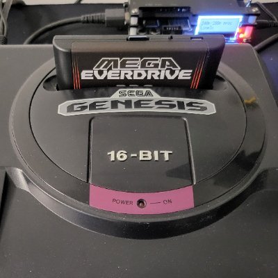
*** SEGA GENESIS/MEGADRIVE - SCALING PART 1 *** I've... been exploring software scaling on the 68k cpu using a background layer rather than scaling sprites. There are a few advantages, no sprite boundaries to worry about so moving pixels is faster also cheaper vertical scaling by adjusting vertical scroll midscreen. The net result is you can manage larger scales more efficiently as the CPU can spend more time working on the horizontal scaling whilst the VDP helps with the vertical scaling (there is still a non trivial cpu cost there though). Here I'm scaling an early image of the Lufthoheit logo - but the goal is to use this in the game also for very large scales / either background effects or bosses. The scaler and Interupt handler are written in Assembly for speed and I think could be faster yet with some optimisations, word alignment moves etc. The scaler has the ability to expand > full screen in height (from a more limited base height) and up to 3x the image width at present. I need to add double buffering and possibly go a bit larger yet. I'm excited to get these effects into the game as large scaling effects we didn't often see on the Genesis ! CYBERDEOUS - Crouzet Laurent Carsten666show more

Free NVIDIA GPU with 16 GB VRAM GPU for... Running Local LLMs! If you want to master local LLMs but you're waiting until you can afford a $1,500 GPU, you're honestly not going to make it. The open source AI ecosystem is moving way too fast for you to wait on your budget to catch up. Especially when you can build a bleeding edge inference engine from scratch right now, completely for free. You don't need a heavy local rig to start. Google is literally letting you use an enterprise grade NVIDIA Tesla T4 GPU for $0/hour. At standard cloud computing rates (~$0.20/hr), Google Colab’s 4 hour daily free tier hands you roughly $24 worth of data center tier GPU compute every single month. And most people just waste it. Let’s talk about the hardware you get access to for free. The NVIDIA Tesla T4 is an absolute workhorse: - Architecture: NVIDIA Turing (TU104) - VRAM: 16GB GDDR6 (320 GB/s bandwidth) - Compute: 320 Tensor Cores | 2560 CUDA Cores - Performance: 130 TOPS INT8 | 8.1 TFLOPS FP32 - Power: Sipping energy at a max 70W TDP This is the exact same hardware I used to run DeepMind's Gemma 4 26B A4B QAT MoE at a 250,000 context window without a single Out Of Memory (OOM) crash. If you have a web browser and 10 minutes, you have everything you need. I’ve put together a fully documented, cell by cell Google Colab notebook that teaches you exactly how to do this. Here is what the notebook actually teaches you: - How to provision an Ubuntu Linux environment with CUDA 13.0 and verify your driver stack. - How to pull the source code and compile the latest llama.cpp C++ binaries from scratch, specifically optimizing the build for your exact GPU using the -DCMAKE_CUDA_ARCHITECTURES=native flag. - How to directly download quantized local LLMs (GGUF format) straight from HuggingFace using the CLI. - How to manage 16GB VRAM limits, offload neural network layers to the GPU, and push massive context windows. Compile raw llama.cpp, ollama run a model, or spin up the LM Studio CLI. Pick whatever stack you are comfortable with. just start building. No hardware. No credit card. No excuses. Bookmark this post right now so you don't lose the tutorial. Even if you don't have time to run it today, you are going to want this workflow in your engineering toolkit. The link to the free Colab Notebook is in the comments below. Lemme know if you need more tutorials like this.show more

my 8 GB VRAM gaming laptop is absolutely going... to hate me for this. but I still did it. ran a 31b dense model (Gemma 4 31b Q4) with only 8 GB VRAM last week I ran Gemma 4 26B A4B a mixture of experts model on my RTX 4060 and hit 25–28 tokens/sec using llama.cpp's new MTP support. smooth. snappy. but MoE has a secret: it only activates 4B parameters per token despite having 26B total. that's why it flies. so the real question started haunting me. what if I throw a full, no tricks, every parameter fires on every token, 31B DENSE model at the same machine? # Hardware: GPU: NVIDIA RTX 4060, 8 GB VRAM RAM: 16 GB CPU: Intel Core i7 H Laptop. Gaming. Modest. The model: gemma-4-31B-it-qat-UD-Q4_K_XL.gguf (model's unsloth huggingface link in the comments) This is Google DeepMind's flagship dense model in the Gemma 4 family that can run on single consumer GPU. It packs a hybrid attention architecture, supports up to 256K context natively, and is QAT (Quantization Aware Training) optimized, meaning it retains far more quality than standard post training quants at the same bit depth. This is NOT the MoE. This is 31 BILLION dense parameters, every single one of them loaded. # the flags I used: -m gemma-4-31B-it-qat-UD-Q4_K_XL.gguf -cnv --spec-type draft-mtp --spec-draft-model mtp-gemma-4-31B-it.gguf --spec-draft-n-max 8 --spec-draft-p-min 0.6 -c 6000 -v Multi Token Prediction (MTP) is still active here. Separate draft GGUF required, same as the 26B setup. # Results: → Decode: ~3 tokens/sec → Prefill: ~2 tokens/sec → Context: 6000 tokens → Hardware crying quietly in the corner: yes so is 3 tps actually usable? For real time back and forth chat? Not ideal. You're not having a fluid conversation at 3 tps. but slow ≠ useless. And this is where it gets genuinely interesting. think about how senior devs actually work in a real team. But when something is architectural, deeply complex, or needs serious reasoning? they walk down the hall and escalate to the senior. That's exactly the local AI agent architecture this unlocks: → Fast orchestrator model (Gemma 4 26B MoE at 25+ tps) handles routing, simple queries, tool calls, memory. The junior dev. → Gemma 4 31B dense is the senior, called only when the fast model genuinely hits a wall. Hard multi step reasoning. Complex code generation. Deep architectural decisions. The agentic loop stays fast. Only the hard hops touch the 31B. That's a legitimate production grade local AI architecture on a budget hardware. (requires 2 8gb gpus) other workflows where 3 tps is completely fine: - overnight batch jobs. summarize documents, extract structured data, review code. Fire it off. Sleep. wake up to results. - One shot deep reasoning - Silent code audit loops, you write and test, the 31B reviews diffs and flags issues in the background between your sprints - Any workflow where output quality > output speed A few weeks ago, nobody was running a 30B+ dense model on a single consumer GPU with 8 GB VRAM. At all. Now we're doing it on an Intel i7-H gaming laptop with a NVIDIA RTX 4060, thanks to llama.cpp + QAT quants + MTP speculative drafting. Google DeepMind said the Gemma 4 31B targets "consumer GPUs and workstations." They were not exaggerating. The hardware bar to run serious frontier class models locally keeps dropping. the tools are here. the models are here. you just have to be willing to abuse your laptop a little. what workflows would you actually run on a local 3 tps 31B dense model? genuinely curious. drop it below.show more

🚨 Anthropic committed up to 1M TPU chips for... Claude. Openai is leasing TPUs for chatgpt inference. Here's How kernels work on TPUs (deep dive 2/6 by emi) pallas is Google's answer to kernel writing. a python kernel SDK built on JAX. still very experimental (jax.experimental.pallas). on TPU it compiles through mosaic; on GPU it lowers to triton. if you know CUDA, the syntax will feel familiar but the execution model is completely different. in CUDA, grid=(4,4) launches 16 blocks running simultaneously across SMs. in pallas, those 16 iterations run one after another in lexicographic order. no threads. no warps. no blocks. no occupancy tuning. a TPU is a sequential machine with a very wide vector register — more like a CPU than a GPU. performance comes from width: a 128x128 systolic array doing matmul and an 8x128 SIMD vector unit doing everything else. maximum parallelism on chip: 2, one per TensorCore in megacore mode. three concepts replace CUDA's thread/block/grid hierarchy. Refs are mutable memory references. because execution is sequential, each iteration safely accumulates without atomics. in CUDA you'd need atomics or a separate reduction pass. the memory model is also very different from NVIDIA's. zero hardware caches. VMEM is 32-128 MiB of software-managed scratchpad — 500-1000x larger than GPU shared memory per SM. all data must be explicitly DMA'd from HBM to VMEM before any computation touches it. four levels: HBM → VMEM → VREGs → MXU/VPU, plus SMEM for scalar control data. every byte of data movement is your responsibility. this is like CUDA shared memory except it's 500x bigger and there's no cache fallback. pipelining is mandatory. without double-buffering HBM→VMEM transfers, the MXU just stalls waiting for data. this is the single most important optimization on TPU. and because grid execution is sequential and deterministic, consecutive iterations that need the same input block skip the redundant HBM transfer automatically, impossible on GPU where block execution order is undefined. the compilation pipeline is unlike anything in this series: python → jaxpr → stableHLO → XLA HLO (71+ optimization passes) → LLO (78+ passes) → 322-bit VLIW bundles. the compiler packs instructions for scalar, vector, matrix, and DMA units into a single 322-bit word. everything in that bundle executes in parallel, with no runtime scheduling.show more

Universities and High Schools have not moved rapidly enough... to guide students to have skills for the next decade. THEY HAVE FAILED. It is a massive crisis that can be averted by understanding what AI and Robotics will bring about. Solutions are knowing how to use these tools and new industries that will rise. But this situation is also on ALL OF US. No “job” is safe from founder to entry level in most industries. You and I, by what we do, will be “replaced” ultimately. What to do? AI and Robotics are tools, the next decade is owned by those who know how to use them expertly, but this is also temporary. We have to understand that what we do for “work” will change giving ultimately a greater value to those that are: Creative Flexible Always learning Willing to be wrong Love being human Love being alive Know history Covet wisdom Knowing all tech has downsides Building strong family and friends Realize many institutions have failed The first four are required for you to be able to live through this period with your sanity intact. The rest will allow you to thrive. There are no true careers at this point anymore. There are advocation and vocations which will either earn you money or give life meaning. We will learn that we are not “what we do”, just like we knew for 99% of human existence. Let that sink in. — You and I are far, far ahead of knowing this and we can do two things: 1) Laugh at the “clueless” 2) Help people understand with grace Go to Reddit if you are 1, in fact don’t follow me because you will not like this next decade and what I post. You are 2 and thank you. Even if you and I have not solved this issue, we can help people understand what is ahead and with determination and creativity bound together to solve it locally. Or human family has done this millions of times. The evidence is: you are here. The Neo Luddite movement has not even begun and it will potentially rip apart society even more than all the fashionable moment in the recent past has. These Luddites will have a good point with the wrong answers cooked up by dying academics that cling to labels, “virtues” and victim hood. It will be readymade for some governments to enter in as “big daddy” to “help us”. You will not like what they do, but you will only know when it is too late. It will include YOU “volunteering” to “leave” by 60, to “help out” CanadaPod style. “Brian, I’m 24 what do I do?”. I hope to do much more here to help. But I do know this: 1) Learn a trade or vocation because it’s valuable. It may also be free to low cost if you do it right. 2) Learn everything you can about USING AI and TRAINING YOUR AI. Your expertise will be in the top 1% for a decade. But not forever. 3) Understand Bitcoin and how it will rise while other things sink. This is a short list for now. We will know more moving forward. When you see videos like this posted below, know one thing: Many of these folks had no real family of mental and physical support. Maybe no parent or one parent. Maybe only a broke system to prepare them for—nothing. This was not their doing. Now it is not your “job” to help them, it is your survival to help them if that is what you need. See some day after the dust settles these 20 year olds will be 40 year olds and running YOUR world. And at some point you may need them more than you think you do. You will need them, as they need you now. THIS IS WHAT PAST WISDOM KNEW. The elders of the past never found the need to piss on the youth and hope for the best. THE YOUTH ARE OUR BEST, let us all find ways to change it, even if every aspect of “the system” wants us to berate them into the ground.show more