Vector Database by Hand ✍️ Vector databases are revolutionizing... how we search and analyze complex data. They have become the backbone of Retrieval Augmented Generation (#RAG). How do vector databases work? [1] Given ↳ A dataset of three sentences, each has 3 words (or tokens) ↳ In practice, a dataset may contain millions or billions of sentences. The max number of tokens may be tens of thousands (e.g., 32,768 mistral-7b). Process "how are you" [2] 🟨 Word Embeddings ↳ For each word, look up corresponding word embedding vector from a table of 22 vectors, where 22 is the vocabulary size. ↳ In practice, the vocabulary size can be tens of thousands. The word embedding dimensions are in the thousands (e.g., 1024, 4096) [3] 🟩 Encoding ↳ Feed the sequence of word embeddings to an encoder to obtain a sequence of feature vectors, one per word. ↳ Here, the encoder is a simple one layer perceptron (linear layer + ReLU) ↳ In practice, the encoder is a transformer or one of its many variants. [4] 🟩 Mean Pooling ↳ Merge the sequence of feature vectors into a single vector using "mean pooling" which is to average across the columns. ↳ The result is a single vector. We often call it "text embeddings" or "sentence embeddings." ↳ Other pooling techniques are possible, such as CLS. But mean pooling is the most common. [5] 🟦 Indexing ↳ Reduce the dimensions of the text embedding vector by a projection matrix. The reduction rate is 50% (4->2). ↳ In practice, the values in this projection matrix is much more random. ↳ The purpose is similar to that of hashing, which is to obtain a short representation to allow faster comparison and retrieval. ↳ The resulting dimension-reduced index vector is saved in the vector storage. [6] Process "who are you" ↳ Repeat [2]-[5] [7] Process "who am I" ↳ Repeat [2]-[5] Now we have indexed our dataset in the vector database. [8] 🟥 Query: "am I you" ↳ Repeat [2]-[5] ↳ The result is a 2-d query vector. [9] 🟥 Dot Products ↳ Take dot product between the query vector and database vectors. They are all 2-d. ↳ The purpose is to use dot product to estimate similarity. ↳ By transposing the query vector, this step becomes a matrix multiplication. [10] 🟥 Nearest Neighbor ↳ Find the largest dot product by linear scan. ↳ The sentence with the highest dot product is "who am I" ↳ In practice, because scanning billions of vectors is slow, we use an Approximate Nearest Neighbor (ANN) algorithm like the Hierarchical Navigable Small Worlds (HNSW).show more

Transformer by hand ✍️ ~ 6 steps walkthrough below... Open the hood of a transformer and the parts list is overwhelming: embeddings, positional encoding, attention weighting, self-attention, cross-attention, multi-head attention, layer norm, skip connections, softmax, linear, Nx, shifted right, query, key, value, masking. Which of those actually make the car run? Two of them. Attention weighting and the feed-forward network. Everything else is an enhancement to make it run faster and longer, which is how we got from a car to a truck, and to the word "large" in large language model. So I drew and calculated those two parts entirely by hand. Goal: push five features through one transformer block, filling in every cell yourself. 1. Given Five positions of input features, arriving from the previous block. 2. Attention matrix Let us feed all five features to a query-key module (QK) and read back an attention weight matrix, A. The details of that module are a post of their own. 3. Attention weighting We multiply the input features by A to get the attention weighted features, Z. Still five positions. The effect is to combine features *across positions*, horizontally: X1 becomes X1 + X2, X2 becomes X2 + X3, and so on. 4. First layer Let us feed all five weighted features into the first layer of the FFN. Multiply by the weights and biases. This time the combining happens *across feature dimensions*, vertically, and each feature grows from 3 numbers to 4. Note that every position goes through the same weight matrix. That is what "position-wise" means. 5. ReLU We cross out the negatives. They become zeros. 6. Second layer Let us bring it back down: 4 dimensions to 3. The output feeds the next block, which has a completely separate set of parameters, and the whole thing runs again. You have just calculated a transformer block by hand. ✍️ The takeaway: the two parts are doing two different jobs, and neither one alone is enough. Attention mixes *across positions*, so a feature can see its neighbours. The FFN mixes *across feature dimensions*, so each position can think about itself. Horizontal, then vertical. Then that pattern repeats N times, each block with its own separate set of weights. That is the Nx from the list up top, and that is what makes the transformer run. 💾 Save this post! #AIbyHand #Transformers #DeepLearningshow more

[Graph Convolutional Network] by hand ✍️ Graph Convolutional Networks... (GCNs), introduced by Thomas Kipf and Max Welling in 2017, have emerged as a powerful tool in the analysis and interpretation of data structured as graphs. This exercise demonstrates how GCN works in a simple application: binary classification. -- Goal -- Predict if a node in a graph is X. -- Architecture -- 🟪 Graph Convolutional Network (GCN) 1. GCN1(4,3) 2. GCN2(3,3) 🟦 Fully Connected Network (FCN) 1. Linear1(3,5) 2. ReLU 3. Linear2(5,1) 4. Sigmoid Simplications: • Adjacent matrices are not normalized. • ReLU is applied to messages directly. -- Walkthrough -- [1] Given ↳ A graph with five nodes A, B, C, D, E [2] 🟩 Adjacency Matrix: Neighbors ↳ Add 1 for each edge to neighbors ↳ Repeat in both directions (e.g., A->C, C->A) ↳ Repeat for both GCN layers [3] 🟩 Adjacency Matrix: Self ↳ Add 1's for each self loop ↳ Equivalent to adding the identity matrix ↳ Repeat for both GCN layers [4] 🟪 GCN1: Messages ↳ Multiply the node embeddings 🟨 with weights and biases ↳ Apply ReLU (negatives → 0) ↳ The result is one message per node [5] 🟪 GCN1: Pooling ↳ Multiply the messages with the adjacent matrix ↳ The purpose is the pool messages from each node's neighbors as well as from the node itself. ↳ The result is a new feature per node [6] 🟪 GCN1: Visualize ↳ For node 1, visualize how messages are pooled to obtain a new feature for better understanding ↳ [3,0,1] + [1,0,0] = [4,0,1] [7] 🟪 GCN2: Messages ↳ Multiply the node features with weights and biases ↳ Apply ReLU (negatives → 0) ↳ The result is one message per node [8] 🟪 GCN2: Pooling ↳ Multiply the messages with the adjacent matrix ↳ The result is a new feature per node [9] 🟪 GCN2: Visualize ↳ For node 3, visualize how messages are pooled to obtain a new feature for better understanding ↳ [1,2,4] + [1,3,5] + [0,0,1] = [2,5,10] [10] 🟦 FCN: Linear 1 + ReLU ↳ Multiply node features with weights and biases ↳ Apply ReLU (negatives → 0) ↳ The result is a new feature per node ↳ Unlike in GCN layers, no messages from other nodes are included. [11] 🟦 FCN: Linear 2 ↳ Multiply node features with weights and biases [12] 🟦 FCN: Sigmoid ↳ Apply the Sigmoid activation function ↳ The purpose is to obtain a probability value for each node ↳ One way to calculate Sigmoid by hand ✍️ is to use the approximation below: • >= 3 → 1 • 0 → 0.5 • <= -3 → 0 -- Outputs -- A: 0 (Very unlikely) B: 1 (Very likely) C: 1 (Very likely) D: 1 (Very likely) E: 0.5 (Neutral)show more

[Discrete Fourier Transform] by Hand ✍️ In signal processing,... the Discrete Fourier Transform (DFT) is no doubt the most important method. But the math involved is extremely complex, literally, involving a summation over a complex number term e^(-iwt). I developed this exercise to demonstrate that underneath such complexity, DFT is just a series of matrix multiplications you can calculate by hand. ✍️ Once you see that, it should not surprise you that a deep neural network, which is also a series of matrix multiplications, with activation functions in-between, can learn to perform DFT to process and analyze signals so effectively. How does DFT work? [1] Given ↳ Signals A, B, and C in the 🟧 frequency domain: ◦ A = cos(w) + 2cos(2w) ◦ B = cos(w) + cos(3w) + cos(4w) ◦ C = -cos(2w) + cos(3w) ◦ Each signal is a weighed sum of four cosine waves at frequencies 1w, 2w, 3w, and 4w. ◦ We will apply Inverse DFT to convert the signals to time domain representations, and then demonstrate DFT can convert back to their original frequency domain representations. ↳ Signal X in the 🟩 time domain. X is sampled at 10 time points 1t, 2t, …, 10t: ◦ X = [-2.5, -1.8, 3, -0.7, -1.0, -0.7, 3, -1.8, -2.5, 5] ◦ Suppose X is also a weighted sum of the same four cosine waves, but we don’t already know their weights. We will apply DFT to discover them. [2] 🟧 Frequency Matrix (F) ↳ Write the coefficients of A, B, C as a matrix F. Each signal is a row. Each frequency is a column. ↳ A → [1, 2, 0, 0] ↳ B → [1, 0, 1, 1] ↳ C → [0, 1-, 1, 0] [3] Cosine → Discrete ↳ Sample from the continuous cosine waves at discrete time points 1t, 2t, 3t, to 10t. [4] Cosine Matrix (W) ↳ Write the samples as a matrix, Each frequency is a row. Each time point is a column. [5] Inverse DFT: 🟧 Frequency → 🟩 Time ↳ Multiply the frequency matrix F and the cosine matrix W. ↳ The meaning of this multiplication is to linearly combine the four cosine waves (rows in W) into time-domain signals (rows in T) using the weights specified in F. ↳ The result is matrix T, which are signals A, B, C converted to the time domain. Each signal is a row. Each time point is a column. [6] Transpose ↳ Transpose T, converting each signal’s time domain representation from a row to a column. [7] DFT: 🟩 Time → 🟧 Frequency ↳ Multiply the cosine matrix W with the transpose of matrix T. ↳ The purpose of this multiplication is to take a dot-product between each time-domain signal (columns in the transpose of T) and each cosine wave (rows in W), which has the effect of projecting the signal onto a cosine wave to determine how much they are correlated. Zero means not correlated at all. ↳ The result is an intermediate version of the “recovered” frequency matrix where each column corresponds to a signal and each row corresponds to a frequency. ↳ Compared to the original frequency matrix F, this intermediate matrix has non-zero weights in the correct places, but scaled up by a factor of 5 (n/2, n=10). For example, signal A, originally [1,2,0,0], is recovered at [5,10,0,0]. [8] Scale ↳ Multiply each value by 2/n = 1/5 to scale down the intermediate matrix to match the magnitude of the original frequency matrix F. [9] Transpose ↳ Transpose the recovered frequency matrix back to the same orientation of the original frequency matrix F. ↳ Like magic 🪄, the result is identical to the original F, which means DFT successfully recovered the frequency components of signals A, B, C. [10] Apply DFT to X: 🟩 Time → 🟧 Frequency ↳ Now that we have some confidence in DFT’s ability to recover frequency components, we apply DFT to X’s time-domain representation by multiplying W with X. ↳ The result is the an intermediate matrix. [11] Scale ↳ Similarly, we scale down by a factor of 5 to obtain the recovered frequency components of X (a column). [12] Transpose ↳ Similarly, we transpose the recovered column to row to match the orientation of the frequency matrix. ↳ Using the coefficients [0,0,3,2], we can write the equation of X as 3cos(3w) + 2cos(4w). Notes: I hope this by hand exercise helps you understand the essence of DFT. But there is more technical details, such as: • Sine: The complete DFT math also includes sine waves that follow a similar calculation process. • Phase: Here, we assume all the cosine waves are aligned at the origin, namely, phase is 0. If a phase p is added, for example, cos(w+p), we will need to calculate the sine component and use their ratio to figure out what p is. • Magnitude: If phase is not zero, the magnitude will need to be calculated by combining both cosine and sine terms.show more

MLP in PyTorch by hand ✍️ ~ 7 steps... walkthrough below Goal: fill in every blank in the PyTorch code to build a multi-layer perceptron. 1. Given Let us start with a code template on the left and the network it is supposed to build on the right. Every blank in the code can be worked out from the picture. 2. Linear layer We count: 3 features in, 4 features out. So the weight matrix is 4 by 3. There is an extra column for the biases, which means bias = T. 3. ReLU Let us apply the activation. ReLU crosses out the negatives, so -1 becomes 0. 4. Linear layer The input size is 4, because that is what the previous layer put out. The output size is 2. A 2 by 4 weight matrix, and this time no extra column, so bias = F. 5. ReLU We cross out the negatives again. 6. Linear layer Two features in, five out. A 5 by 2 weight matrix, with a bias column, so bias = T. 7. Sigmoid Let us finish. Sigmoid squashes the raw scores (3, 0, -2, 5, -5) into probabilities between 0 and 1. You have just implemented a three-layer deep neural network by hand. ✍️ == Story == Three years ago I gave this exercise to my students, to connect the code to the math. They found it odd. Every other AI course they were taking lived inside a Jupyter notebook, and here I was handing out paper. Three years later, my colleagues are the ones rushing to move their materials to paper. The exercise has not changed. Paper still asks the one thing a notebook lets you skip: do you actually understand what the code is doing? If you can tell me why the weight matrix is 4 by 3, and why bias is F on the second layer, you understand nn.Linear better than someone who has been copy-pasting it for a year. 💾 Save this post! #AIbyHand #PyTorch #DeepLearningshow more

[VAE] by Hand ✍️ A Variational Auto Encoder (VAE)... learns the structure (mean and variance) of hidden features and generates new data from the learned structure. In contrast, GANs only learn to generate new data to fool a discriminator; they may not necessarily know the underlying structure of the data. The International Conference on Learning Representations (ICLR) this year announced its first ever "Test of Time Award" to recognizes the VAE paper, published 10 years ago. This exercise demonstrates how to calculate a VAE by hand. [1] Given: ↳ Three training examples X1, X2, X3 ↳ Copy training examples to the bottom ↳ The purpose is to train the network to reconstruct the training examples. ↳ Since each target is a training example itself, we use the Greek word "auto" which means "self." This crucial step is what makes an autoencoder "auto." [2] Encoder: Layer 1 + ReLU ↳ Multiply inputs with weights and biases ↳ Apply ReLU, crossing out negative values (-1 -> 0) [3] Encoder: Mean and Variance ↳ Multiply features with two sets of weights and biases ↳ 🟩 The first set predicts the means (𝜇) of latent distributions ↳ 🟪 The second set predicts the standard deviation (𝜎) of latent distributions [4] Reparameterization Trick: Random Offset ↳ Sample epsilon ε from the normal distribution with mean = 0 and variance = 1. ↳ The purpose is to randomly pick a offset away from the mean. ↳ Multiply the standard deviation values with epsilon values. ↳ The purpose is to scale the offset by the standard deviation. [5] Reparameterization Trick: Mean + Offset ↳ Add the sampled offset to predicted mean ↳ The result are new parameters or features 🟨 as inputs to the Decoder. [6] Decoder: Layer 1 + ReLU ↳ Multiply input features with weights and biases ↳ Apply ReLU, crossing out negative values. Here, -4 is crossed out. [7] Decoder: Layer 2 ↳ Multiply features with weights and biases ↳ The output is Decoder's attempt to reconstruct the input data X from reparameterized distributions described by 𝜇 and 𝜎. [8]-[10] KL Divergence Loss [8] Loss Gradient: Mean 𝜇 ↳ We want 𝜇 to approach 0. ↳ A lot of math called SGVB simplifies the calculation of loss gradients to simply 𝜇 [9,10] Loss Gradient: Stdev 𝜎 ↳ We want 𝜎 to approach 1. ↳ A lot of math simplifies the calculation to 𝜎 - (1/ 𝜎) [11] Reconstruction Loss ↳ We want the reconstructed data Y (dark 🟧) to be the same as the input data X. ↳ Some math involving Mean Square Error simplifies the calculation to Y - X.show more

One cool thing about ColBERT-based search compared to the... cosine-based vector retrieval is that you get interpretability for free as a byproduct of the MaxSim computation. It's kind of like the Lucene highlighter, letting you grab the most relevant snippets from a long document to show users where their query matches. With Jina-ColBERT-v1, which supports up to 8K token length, released by us earlier this Feb., the visualization of the late interaction between a query and a document is almost... artistic. The video shows the late interaction between the query "Elephants eat 150 kg of food per day." and the Wikipedia article about "Indian Elephant". Darker colors indicate stronger semantic matches. The darkest area corresponds to "The species is classified as a megaherbivore and consume up to 150 kg (330 lb) of plant matter per day." from the original article.show more

A good technical LLM interview question: Your RAG chatbot... is working as expected locally. You deploy it behind a load balancer with 3 replicas. Users report that it forgets what they just asked, and answers get worse with each restart. Why did this happen? (answer below) A local setup has one process that owns everything. - The vector index is a variable in memory. - Conversation history is a Python list. - The documents are on local disk. You never treat any of them as infrastructure, because restarting rebuilds all three in seconds and there is only ever one copy. The setup does not carry over to production directly. The vector index might disappear on restart, so the app re-embeds everything on boot and serves empty results until it finishes. Conversation history may belong to one replica, so a follow-up routed elsewhere has no memory of the previous turn. Documents could be on whichever container ingested them, so the three replicas hold three different corpora. None of this is evident with one user and one process. So the actual work in shipping RAG is not just the retrieval logic, but also storing the vector index, the conversation history, and the documents outside the app, where every replica reads and writes the same copy. Which comes down to three requirements: > The vector store needs persistence and has to be reachable from every replica. pgvector inside Postgres keeps embeddings next to the rest of the data instead of adding another system to operate. > Conversation state has to be checkpointed outside the app. LangGraph writes its state to Postgres, so any replica can pick up a thread mid-conversation. > Docs need shared object storage, so ingestion happens once instead of once per replica. If you get those three right, the retrieval logic you wrote in the notebook works unchanged. To learn how all of it is wired together, Akamai's GitHub has a working reference implementation. - rag-langgraph-k8s-quickstart is an airline policy Q&A assistant built with FastAPI, LangChain, and LangGraph. Terraform provisions the LKE cluster, a Postgres instance with pgvector for embeddings, a second Postgres for LangGraph checkpointing, and an object storage bucket for the policy documents, in one apply. - akamai-workshop-ai-inference covers the next step, running the model yourself instead of calling an API, with prefill and decode, KV cache tradeoffs, and continuous batching under real concurrency. Both are available on Akamai's new Developer Hub, alongside their tutorials and code samples. It also links to Edge Case, their Discord, where four developer advocates architect and deploy a production app live every other Wednesday. If you create a new Akamai Cloud account, you can also get $300 in credits for joining. Join here: That said, this post assumes the retrieval logic was right to begin with, and that is doing a lot of work. Most RAG systems fail earlier, at the point where a chunk gets treated as a self-contained unit of meaning. I wrote about the two skills that fix that gap, and why the chunk is usually the wrong thing to embed. Read it below. Thanks to Akamai Cloud for partnering today!show more

[Deep RNN] by Hand ✍️ A Deep Recurrent Neural... Network (RNN) extends a basic single-layer RNN into multiple layers of hidden states, effectively incorporating deep learning into the RNN architecture. How does a Deep RNN work? [1] Given ↳ A sequence of four inputs X1, X2, X3, X4 ⬛️ ↳ Recurrent weights and biases for hidden layers a 🟩, b 🟧, c 🟪, and the output layer y 🟦. [2] Initialize Hidden States ↳ Set a0, b0, c0 to zeros — Process X1 (t = 1)— [3] First Hidden Layer (a) 🟩: a0 → a1 ↳ The transformation matrix is horizontal concatenation of input weights, hidden state weights and biases, visualized as [⬛️ | 🟩 | ⬜️] . ↳ The state matrix is vertical concatenation of input X1, previous hidden state a0, and an extra 1, visualized as [⬛️ ; 🟩 ; 1]. ↳ Multiply the two matrices to obtain new hidden state a1 = [0 ; 1]. [4] Second Hidden Layer (b) 🟪: b0 → b1 ↳ First layer a1 🟩 becomes the input. ↳ The transformation matrix is visualized as [🟩 | 🟪 | ⬜️]. ↳ The state matrix is the combination of a1, b0, and 1, visualized as [🟩; 🟪 ; 1]. ↳ Multiply the two matrices to obtain new hidden state b1 = [1; -1]. [5] Third Hidden Layer (c) 🟧: c0 → c1 ↳ Second layer b 🟪 becomes the input. ↳ The transformation matrix is visualized as [🟪 | 🟧 | ⬜️]. ↳ The state matrix is the combination of a1, b0, and 1, visualized as [🟪; 🟧; 1]. ↳ Multiply the two matrices to obtain new hidden state b1 = [1; -1]. [6] Output Layer (Y) 🟦 ↳ The transformation matrix is visualized as [🟧 | ⬜️]. ↳ The state matrix is the combination of c0 and , visualized as [🟧; 1]. ↳ Multiply the two matrices to obtain output Y1 = [3; 0; 3]. — Process X2 (t = 2)— [7] Previous Hidden States ↳ Copy the values of a1, b1, c1. [8] Hidden 🟩🟪🟧 + Output 🟦 ↳ Repeat [3]-[6] to obtain output Y2 = [5; 0; 4] — Process X3 (t = 3)— [9] Previous Hidden States ↳ Copy the values of a2, b2, c2. [10] Hidden 🟩🟪🟧 + Output 🟦 ↳ Repeat [3]-[6] to obtain output Y3 = [13; -1; 9] — Process X4 (t = 4)— [11] Previous Hidden States ↳ Copy the values of a3, b3, c3. [12] Hidden 🟩🟪🟧 + Output 🟦 ↳ Repeat [3]-[6] to obtain output Y4 = [15; 7; 2]show more

Researchers made KMeans 200x faster. And the new technique... also beats approaches like cuML and FAISS. Flash-KMeans is an IO-aware implementation of exact KMeans that redesigns the algorithm around modern GPU bottlenecks. By attacking the memory bottlenecks directly, Flash-KMeans achieves: - 33x speedup over cuML - 200x speedup over FAISS This speedup comes from how it moves through GPU memory. Standard KMeans runs in two steps, and both are bottlenecked by reads and writes to GPU memory: 1) The first step matches every point to its nearest centroid. Standard KMeans computes the full point-to-centroid distance matrix, writes it out to GPU memory, then reads it back to find each nearest centroid. That write-then-read round trip is the bottleneck. Flash-KMeans combines the distance calculation with the nearest-centroid step, so the result is computed on-chip and the full matrix is never written out. 2) The second step recomputes each centroid by averaging the points assigned to it. Standard KMeans has thousands of threads writing into the same centroid slots at once, so they stall waiting for their turn. Flash-KMeans sorts points by cluster first, turning scattered writes into sequential reductions that read and write memory in one efficient pass. Using these two optimizations at the million-scale, Flash-KMeans completes a standard KMeans iteration in a few milliseconds. The video below depicts this in action. Several reasons why this is important: KMeans has always been an offline primitive. Something you run once to preprocess data and move on. These speedups make the approach viable in several runtime-critical systems. ↳ Vector indices like FAISS use KMeans to build search indices. Faster KMeans means you can re-index dynamically as data changes. ↳ LLM quantization methods need KMeans to find optimal weight codebooks, per layer, repeatedly. What takes hours could now take minutes. ↳ MoE models need fast token routing at inference time. Flash-KMeans makes it viable to run this inside the inference loop, not just in preprocessing. I have shared the paper in the replies. That said, memory is the real constraint Flash-KMeans solves, and the problem is not just limited to clustering. The vectors a RAG system stores after indexing create similar bottlenecks. I wrote a detailed walkthrough recently on cutting this vector memory by 32x with binary quantization, querying 36M+ vectors in a few milliseconds. Read it below.show more

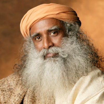
Kedarnath is a tremendous space. The utterance of the... sound “Shiva” attains a completely new dimension and significance in Kedar. It is a space which has been specially prepared for this particular sound. When we utter the word “Shiva,” it is the freedom of the uncreated, the liberation of one who is not created. It is almost like on this planet, the sound “Shiva” emanates from this place. For thousands of years, people have experienced that space as a reverberation of that sound. This is also a place that has witnessed thousands of Yogis and mystics of every kind. When I say every kind, you cannot imagine those kinds. These are people who made no attempt to teach anything to anyone. Their way of making an offering to the world was by leaving their energies, their path, their work – everything – in a certain way in these spaces.show more

As a gynecologist, one of the most frequently asked... questions is about the ''hymen''. The hymen is not a structure located deep inside the vagina. It is a thin, flexible fold of tissue situated very close to the vaginal opening, anatomically at the entrance of the vaginal canal. It is typically found about 1–2 cm inside the vaginal opening, but in many women, it is almost at the surface. Therefore, the common belief that it is located deep inside is incorrect. One of the most important points is this: The hymen is not a closed membrane. It naturally has openings that allow menstrual blood to pass. Additionally, the structure of the hymen varies from person to person. Its thickness, elasticity, and shape are not standard. In some women, it may be very thin and elastic, while in others, it may be minimal or barely noticeable. This is completely a normal anatomical variation. A common misconception is that changes in the hymen occur only due to sexual intercourse. In reality, factors such as certain physical activities or tampon use can also lead to stretching or changes in this tissue. Therefore, the hymen is not a reliable indicator of a person’s sexual history or “virginity.” In summary, the hymen is a small and variable anatomical structure. The meanings attributed to it are largely shaped by sociocultural beliefs rather than medical facts.show more

The UFO/UAP phenomenon is ancient. It has been here... long before us, and it is connected to a grand hierarchy created by God. They are coming from higher dimensions, something that religions would describe as the Tree of Life. The phenomenon is part of us, and our soul is part of this grand system. We are currently in the lowest dimension, chakra, sefirot, or part of the soul, known as Malkhut in Kabbalah, Muladhara in Hinduism, and Khat in ancient Egypt. We are made of matter, but our soul is made of fire, and it is time for an upgrade. The Geophysical Event is connected to this transformation.show more

[LSTM] by Hand ✍️ LSTMs have been the most... effective architecture to process long sequences of data, until our world was taken over by the Transformers. LSTMs belong to the broader family of recurrent neural network (RNNs) that process data sequentially in a recurrent manner. Transformers, on the other hand, abandon recurrence and use self-attention instead to process data concurrently in parallel. Recently, there is renewed interest in recurrence as people realized self-attention doesn’t scale to extremely long sequences, like hundreds of thousands of tokens. Mamba is a good example to bring back recurrence. All of a sudden, it is cool to study LSTMs. How do LSTMs work? [1] Given ↳ 🟨 Input sequence X1, X2, X3 (d = 3) ↳ 🟩 Hidden state h (d = 2) ↳ 🟦 Memory C (d = 2) ↳ Weight matrices Wf, Wc, Wi, Wo Process t = 1 [2] Initialize ↳ Randomly set the previous hidden state h0 to [1, 1] and memory cells C0 to [0.3, -0.5] [3] Linear Transform ↳ Multiply the four weight matrices with the concatenation of current input (X1) and the previous hidden state (h0). ↳ The results are feature values, each is a linear combination of the current input and hidden state. [4] Non-linear Transform ↳ Apply sigmoid σ to obtain gate values (between 0 and 1). • Forget gate (f1): [-4, -6] → [0, 0] • Input gate (i1): [6, 4] → [1, 1] • Output gate (o1): [4, -5] → [1, 0] ↳ Apply tanh to obtain candidate memory values (between -1 and 1) • Candidate memory (C’1): [1, -6] → [0.8, -1] [5] Update Memory ↳ Forget (C0 .* f1): Element-wise multiply the current memory with forget gate values. ↳ Input (C’1 .* o1): Element-wise multiply the “candidate” memory with input gate values. ↳ Update the memory to C1 by adding the two terms above: C0 .* f1 + C’1 .* o1 = C1 [6] Candiate Output ↳ Apply tanh to the new memory C1 to obtain candidate output o’1. [0.8, -1] → [0.7, -0.8] [7] Update Hidden State ↳ Output (o’1 .* o1 → h1): Element-wise multiply the candidate output with the output gate. ↳ The result is updated hidden state h1 ↳ Also, it is the first output. Process t = 2 [8] Initialize ↳ Copy previous hidden state h1 and memory C1 [9] Linear Transform ↳ Repeat [3] [10] Update Memory (C2) ↳ Repeat [4] and [5] [11] Update Hidden State (h2) ↳ Repeat [6] and [7] Process t = 3 [12] Initialize ↳ Copy previous hidden state h2 and memory C2 [13] Linear Transform ↳ Repeat [3] [14] Update Memory (C3) ↳ Repeat [4] and [5] [15] Update Hidden State (h3) ↳ Repeat [6] and [7]show more

I built MatmulFlow ( — an interactive tool that... makes matrix multiplication dimensions visual, part of my AI by Hand ✍️ series. Matrix multiplication dimensions are confusing. Which is the inner dimension? Columns of the first or rows of the second? And when you chain five multiplications together, it gets worse. The idea: represent matrices as rectangles. Shift the second matrix up and to the right. The edges that must align become obvious. The result fills in the remaining space. No memorization. You can see it. It extends to chains. Stack vertically for left-multiplication. Stack horizontally for right-multiplication. Resize any matrix and watch the dimensions "flow" through the entire chain. Give it a try!show more

The Hidden Language of Diffusion Models paper page: tackle... the challenge of understanding concept representations in text-to-image models by decomposing an input text prompt into a small set of interpretable elements. This is achieved by learning a pseudo-token that is a sparse weighted combination of tokens from the model's vocabulary, with the objective of reconstructing the images generated for the given concept. Applied over the state-of-the-art Stable Diffusion model, this decomposition reveals non-trivial and surprising structures in the representations of concepts. For example, we find that some concepts such as "a president" or "a composer" are dominated by specific instances (e.g., "Obama", "Biden") and their interpolations. Other concepts, such as "happiness" combine associated terms that can be concrete ("family", "laughter") or abstract ("friendship", "emotion"). In addition to peering into the inner workings of Stable Diffusion, our method also enables applications such as single-image decomposition to tokens, bias detection and mitigation, and semantic image manipulationshow more

Added context to my tiny diffusion model to enable... sequential generation of longer outputs! Currently the context is a quarter of the sequence length (seq_len=256, context_len=64). I have a theory that the less semantic-value-per-token, the worse the “curse of parallel decoding” is. With parallel decoding, we independently predict multiple tokens in one step. With the sentence “My poker hand was a ___ ___”, two valid predictions are “two pair” and “straight flush”. Because each token prediction is independent though, we can end up with a nonsensical output like “two flush”. This seems to be exacerbated with low semantic-value-per-token, as now you need more tokens to express the same concept. Instead of needing to independently predict two tokens, we might need to predict 10 instead (which is of course much harder). The model currently has noticeably worse output compared to nanogpt (similar size) and I believe this is a main reason. I’ll try adding confidence-aware parallel decoding (from NVIDIA’s Fast-dLLM paper) and other tricks and see how much they improve generation quality.show more

If you are an USM student, Alumni, Fan, or... a resident of the Pinebelt/surrounding areas you need to be at The Rock this Saturday vs Texas State, and in 2 weeks vs Troy. The Eags are 7-2. They are 5-0 in the Sunbelt. People have wanted a winning product, and Huff has delivered by flipping a 1-11 team over night basically. The Eags not only have a chance to win the west, and play for a conference championship. But win out and with some help there is a small outside chance of being the G5 team in the playoffs. Which is crazy to say, but it’s not impossible. The team is fun to watch, and KujForCongress brings the energy to make it a good time for everyone. Don’t miss out! Need tickets call Tyler Cochran ! #SMTTTshow more

As someone who is pretty up to date in... AI I’d say there are 2 times a year where I am genuinely blown away by something. A breakthrough that keeps me up at night. This is one of them. I mean the video of will smith genuinely freaks me out by how good it is. 2.5 years of AI progress and you think it’s hitting a wall. There’s no point in trying to convince people where this is going. The writing is on the wall. I can bring a horse to water but I can’t force him to drink.show more