正在加载视频...

视频加载失败

Bertrand’s Theorem states that only two central forces close every bounded orbit: F(r) ∝ - 1/r² and F(r) ∝ - r. The first gives the familiar Keplerian ellipses of Newtonian gravity. The second is the isotropic harmonic oscillator. Other central forces can still conserve energy and angular momentum, but...

16,951 次观看 • 4 天前 •via X (Twitter)

0 条评论

暂无评论

原始帖子的评论将显示在这里

相关视频

Physics feels stable, predictable, and well-behaved largely because we learned it in 3D. That comfort hides a trap. In 1907, Paul Ehrenfest pointed out something unsettling. If you take the laws we treat as fundamental and transplant them into a different number of spatial dimensions, they often stop working the way we expect. Not just numerically different but qualitatively different. The issue isn’t the force law by itself. It’s geometry. Gauss’s law ties inverse-square forces to the surface area of spheres, and sphere geometry depends on dimension. Change the dimension, and the same-looking force produces a different potential, a different balance of attraction and inertia, and a different fate for motion. You can see this cleanly with a single problem of central force motion. In d spatial dimensions, flux conservation gives F(r) ∝ 1 / rᵈ⁻¹ so the potential scales as V(r) ∝ −1 / rᵈ⁻² (for d ≠ 2) Now add angular momentum. The effective radial potential becomes V_eff(r) = L² / (2 m r²) − C / rᵈ⁻² In 3D, those two terms balance in just the right way to allow stable bound orbits. Small perturbations stay small. Atoms don’t collapse. Planets don’t spiral away. In other dimensions, that balance breaks. In 2D, the force becomes 1/r, the potential becomes logarithmic, and bound motion sits on a knife edge. In 4D and higher, the attractive term becomes too steep. The centrifugal barrier loses the fight. Orbits plunge or escape. Same equations. Same initial conditions. Different dimension. Different physics. This isn’t science fiction. It’s a warning label. So it's clear that a lot of what we call physical intuition is really three-dimensional intuition wearing a lab coat. #Physics #MathematicalPhysics #ClassicalMechanics #DynamicalSystems #Geometry #Ehrenfest

Mathelirium

32,138 次观看 • 5 个月前

Quantum Mechanics Series Lecture 4 Lecture 1 established that ρ(x,t) = |ψ(x,t)|² behaves like a conserved probability density. Lecture 2 showed what drives that flow. We also saw that writing ψ = r exp(iθ) makes the probability current proportional to the phase gradient, making it clear that phase geometry literally steers the motion. Lecture 3 then showed that the centroid of that flow can move almost classically when the packet is tight and the external potential is smooth. However, that raises yet another question. If the centroid can look classical, why does the full wave still spread, bend, split, and interfere in ways no classical particle cloud would? This is because the wave is not driven only by the external potential. It is also driven by its own curvature. Write ψ(x,t) = r(x,t) exp(iθ(x,t)) with ρ = r². Then Schrödinger’s equation gives two coupled real equations. One is the continuity equation you already know. The other looks like a Hamilton-Jacobi equation, but with one extra term: Q = −(1/2m) ∇²r / r This is the so-called Quantum Potential. It depends entirely on how the amplitude bends across space. So, the wave is being shaped not only by V(x,t), but also by the geometry of its own envelope. In the animation, the upper surface is still |ψ| and its skin is still colored by arg(ψ). The glowing threads still trace the probability current. But now a second membrane hangs underneath. That lower membrane encodes the quantum potential Q itself. The porcelain bead marks the quantum centroid. The amber bead follows a classical centroid under the same external V. When those paths separate, the lower membrane tells you why. The difference is not magic but the extra term classical mechanics does not have. The math breakdown: Start from Schrödinger evolution in units with ħ = 1: i ∂ψ/∂t = [ −(1/2m) ∇² + V(x,t) ] ψ Write the state in polar form: ψ = r exp(iθ) Then ρ = |ψ|² = r² From the imaginary part, you recover probability conservation: ∂ρ/∂t + ∇·j = 0 with j = (1/m) Im(ψ* ∇ψ) = (ρ/m) ∇θ So the local velocity field is v = j / ρ = ∇θ / m Now take the real part of Schrödinger’s equation. That gives ∂θ/∂t + |∇θ|² / (2m) + V + Q = 0 where Q = −(1/2m) ∇²r / r This is the classical Hamilton-Jacobi equation with one extra term. That extra term is what makes quantum motion locally different from classical motion. Take a gradient of that phase equation and use v = ∇θ / m. Then the flow obeys an Euler-like equation: ∂v/∂t + (v·∇)v = −(1/m) ∇(V + Q) In other words, there are really two forces in the problem. One comes from the external potential V. The other comes from the wave’s own curvature through Q. That is why Ehrenfest is only approximate. The centroid can still satisfy d⟨x⟩/dt = ⟨p⟩/m d⟨p⟩/dt = −⟨∇V⟩ but the internal shape of the packet evolves under the combined influence of V and Q. When the packet stays broad and smooth, Q is gentle and the motion looks more classical. When the packet develops sharp curvature or interference structure, Q becomes strong and the classical picture breaks down. That is what this scene is designed to show live. #QuantumMechanics #Wavefunction #SchrodingerEquation #BornRule #ProbabilityCurrent #ContinuityEquation #Phase #EhrenfestTheorem #QuantumPotential #Madelung #HamiltonJacobi #MathematicalPhysics #Mathematics #Physics

Mathelirium

20,456 次观看 • 3 个月前

Quantum mechanics has a reputation for being mystical mainly because people skip the rules and jump to interpretations. In this lecture series, we’re doing the opposite. We start from the rules, follow the algebra, and let the picture be the calculation. Classical Probability Theory combines alternatives by adding their probabilities. Quantum Theory combines them one step earlier…add complex amplitudes first, then square at the end. That swap in order is everything. Expand |a₁ + a₂|² and you don’t just get |a₁|² + |a₂|²…you get a cross-term, 2 Re(a₁ a₂*). Its sign is set by phase, so the same two contributions can reinforce or cancel. Interference is just the algebra of squaring a sum. In the 3D render, the surface height is proportional to |a(x)| (so peaks become bright bands after squaring), while the surface skin is colored by the local phase arg(a(x)). As the phase knob φ(t) is swept on path 2, the cross-term oscillates, and you literally watch the interference ridges slide across the screen. We model a detector screen with coordinates x in R² (think x = (x,y)). A quantum state assigns a complex amplitude a(x). The rule for outcomes is p(x) = |a(x)|² Now the key situation: two coherent alternatives contribute to the same outcome x. Let their amplitudes be a₁(x) and a₂(x). Quantum says a(x) = a₁(x) + a₂(x) So the probability density becomes p(x) = |a₁(x) + a₂(x)|² Expand it (this is the whole episode): p(x) = (a₁ + a₂)(a₁* + a₂*) = |a₁|² + |a₂|² + a₁ a₂* + a₁* a₂ = |a₁|² + |a₂|² + 2 Re(a₁ a₂*) That last term is the interference term. It can be positive or negative. To see phase explicitly, write each contribution in polar form: a₁(x) = r₁(x) exp(i θ₁(x)) a₂(x) = r₂(x) exp(i θ₂(x)) Then a₁ a₂* = r₁ r₂ exp(i(θ₁ − θ₂)) So the cross-term is 2 Re(a₁ a₂*) = 2 r₁ r₂ cos(θ₁(x) − θ₂(x)) That’s the fringe engine: p(x) = r₁² + r₂² + 2 r₁ r₂ cos(Δθ(x)) Now the phase knob we animate: Add a controllable phase shift φ to path 2: a₂(x) → a₂(x) exp(i φ) Then Δθ(x) → Δθ(x) − φ, so p(x; φ) = r₁² + r₂² + 2 r₁ r₂ cos(Δθ(x) − φ) As φ changes smoothly, the bright/dark pattern slides continuously. Same setup, same geometry, same magnitudes r₁,r₂, only phase changed. #QuantumMechanics #WaveInterference #ComplexAmplitudes #DoubleSlit #Physics #Mathematics

Mathelirium

81,501 次观看 • 6 个月前

Thank you for taking the time to write this up — and for the pointer to your thesis; that figure is beautiful. You're right that classical sphere inversion is exactly the starting point: the feature is named "Sphere Inversion" in the tool for that reason. "Inversphere" is the name of the resulting object, not a claim of new mathematics. I should say up front that I'm not a mathematician, so please correct me if I get any of this wrong. My motivation was visual rather than mathematical: with the classical map, the entire far field piles up into a dense blob at the center (10× farther ⇒ 10× closer), and I simply wanted to control that density to balance the look of the finished object. To do that, the radial profile is generalized to f(r) = R·h(v), where v = (R/r − R/D)/(1 − R/D) is a normalized inverted depth and h is a μ-law log compression, h(v) = ln(1+μv)/ln(1+μ). Classical R²/r is the special case μ = 0, D = ∞. The footage here uses μ > 0, so — as far as I can tell — the map shown is outside the conformal family: the tangential scale f/r and radial scale |f′| agree only in the classical limit. If I understand Liouville's theorem correctly, this trade-off was unavoidable: staying conformal in 3D leaves no freedom to adjust the density, so angle preservation is given up deliberately in exchange for control over it. With μ > 0, mid-field depth below the sphere surface grows like log r, so distant scenery layers logarithmically inside the sphere. The 3DGS side also needed some care: each splat's covariance is carried by the Jacobian J = s·I + (f′−s)nnᵀ, depth sorting has to be re-keyed because inversion reverses the radial order, and the on/off transition is a linear blend whose Jacobian is exactly mix(I, J, t). Thanks again for taking the time — an expert eye on this is very welcome.

VoxelKei

30,164 次观看 • 5 天前

Do you actually know what convex optimization is in the geometric, guarantee-theoretic sense or have you only met it through solvers and loss curves? Convexity is rare comfort in optimization...there are no spurious local minima, no surprise traps, and inequalities you can use like tools instead of prayers. So, what is this convexity? Let x = (x₁, x₂) and let f(x) be convex. Plot the surface z = f(x). Pick a contact point x₀. The local slope is the gradient p = ∇f(x₀). That p is exactly the data that defines the supporting plane: z = f(x₀) + p · (x − x₀). Thus, f is said to be convex because for every x, f(x) ≥ f(x₀) + p · (x − x₀). So the plane at x₀ can slide under the surface, but it never slices through it. Not near the point...everywhere. Now for here is the interesting part: The slope becomes a coordinate system! Rewrite the same plane as z = p · x − b, where b is the offset. Because the plane passes through (x₀, f(x₀)), the offset is forced to be b = p · x₀ − f(x₀). And that number isn’t just geometry trivia. It’s the convex conjugate: f*(p) = sup over x ( p · x − f(x) ). At a differentiable contact point, the supporting plane touches f tightly enough that the supremum is achieved at x₀, giving the identity f*(p) = p · x₀ − f(x₀) when p = ∇f(x₀). So one moving contact point gives two linked readouts: primal position x₀ dual position (slope) p = ∇f(x₀) dual offset f*(p) One surface. Two worlds. #ConvexOptimization #Optimization #MachineLearning #SignalProcessing #AppliedMath #Engineering

Mathelirium

38,506 次观看 • 6 个月前