Video yükleniyor...

Video Yüklenemedi

Ana Sayfaya Dön

Lanterns on the Logarithmic Sea Zeros and poles of a complex rational function R(z,t) drift across a 3D landscape carved from the logarithmic potential U(z,t)=log|R(z,t)|. Every ridge, valley, and glowing thread comes from the moving R(z,t), while the particles follow the tangent field of its level curves. The golden...

14,941 görüntüleme • 16 gün önce •via X (Twitter)

0 Yorum

Yorum bulunmuyor

Orijinal gönderinin yorumları burada görünecek

Benzer Videolar

Lecture 1 on Physics-Informed Neural Networks: A Mini-Series Physics-Informed Neural Networks (PINNs) are neural networks trained to satisfy a differential equation by building the PDE residual directly into the loss. They emerged from a very practical problem...classical PDE pipelines can be brilliant, but they often demand heavy discretization work (meshes, stencils, stability tuning), and the method you build is usually tied to one geometry and one solver setup. A PINN flips the workflow by representing the solution itself as a smooth function uᵩ(x,t) and enforcing the physics everywhere you choose to sample the domain. People often meet PINNs in the least helpful way...via a flashy solution plot, and almost no explanation of what was enforced to get it. In this series we keep the enforcement visible. We pick a differential equation, represent the unknown solution as a flexible function, measure how well that function satisfies the equation across the domain, and train it to reduce that mismatch everywhere we sample. A normal neural net learns from labels...you give it inputs and target outputs. A PINN learns from a differential equation...you give it inputs (x,t) and it gets punished whenever its output fails the PDE. By punish we mean that the loss increases when the mismatch is large we reward it if the loss decreases as the mismatch gets smaller. The network isn’t replacing physics, it’s becoming a flexible function that is forced to satisfy the same calculus you’d impose on any candidate solution. The math breakdown: We start with a PDE we want to solve on a domain Ω. Write it as uₜ(x,t) + N(u(x,t), uₓ(x,t), uₓₓ(x,t), …) = 0 for (x,t) in Ω A PINN replaces the unknown function u with a neural network output uᵩ(x,t) Now define the physics residual by plugging uᵩ into the PDE rᵩ(x,t) = ∂uᵩ/∂t + N(uᵩ, ∂uᵩ/∂x, ∂²uᵩ/∂x², …) If uᵩ were an exact solution, we would have rᵩ(x,t) = 0 everywhere. We may also have data points (xᵢ,tᵢ,uᵢ) from measurements or a known initial condition. The training objective is just a weighted sum of squared errors L(ᵩ) = L_data(ᵩ) + λ L_phys(ᵩ) + L_bc/ic(ᵩ) with L_data(ᵩ) = meanᵢ |uᵩ(xᵢ,tᵢ) − uᵢ|² L_phys(ᵩ) = meanⱼ |rᵩ(xⱼ,tⱼ)|² where (xⱼ,tⱼ) are the collocation points in Ω L_bc/ic(ᵩ) = penalties enforcing boundary conditions and initial conditions The key technical step is that the derivatives inside rᵩ are computed by automatic differentiation ∂uᵩ/∂t, ∂uᵩ/∂x, ∂²uᵩ/∂x², … So we can differentiate the total loss L(ᵩ) with respect to ᵩ and train with gradient descent. This is the whole idea behind PINNs. Learn a function, but make the PDE part of the loss, so the network is trained to be a solution, not just a curve-fitter. In the render, the main 3D surface is the network’s current guess uᵩ(x,t), drawn as a living sheet over the (x,t) plane. Hovering above is the neural scaffold...a visible graph of feature nodes and connections. The bright tension threads are the physics residual rᵩ(x,t): each thread tethers a collocation bead on the sheet up to the scaffold, and it thickens and brightens exactly where |rᵩ| is large (color encodes the sign). As training runs, those threads go slack across the domain not because we hid the error, but because the network has actually been pushed toward rᵩ(x,t) ≈ 0. #PINNs #PhysicsInformedNeuralNetworks #ScientificMachineLearning #PDE #DifferentialEquations #Optimization #MachineLearning #AppliedMath #ComputationalPhysics

Mathelirium

47,308 görüntüleme • 5 ay önce

What if Your Neural Network Was Forced to Obey Physics? Physics-Informed Neural Networks (PINNs) are neural networks trained to satisfy a differential equation by building the PDE residual directly into the loss. They emerged from a very practical problem...classical PDE pipelines can be brilliant, but they often demand heavy discretization work (meshes, stencils, stability tuning), and the method you build is usually tied to one geometry and one solver setup. A PINN flips the workflow by representing the solution itself as a smooth function uᵩ(x,t) and enforcing the physics everywhere you choose to sample the domain. People often meet PINNs in the least helpful way...via a flashy solution plot, and almost no explanation of what was enforced to get it. In this series we keep the enforcement visible. We pick a differential equation, represent the unknown solution as a flexible function, measure how well that function satisfies the equation across the domain, and train it to reduce that mismatch everywhere we sample. A normal neural net learns from labels...you give it inputs and target outputs. A PINN learns from a differential equation...you give it inputs (x,t) and it gets punished whenever its output fails the PDE. By punish we mean that the loss increases when the mismatch is large we reward it if the loss decreases as the mismatch gets smaller. The network isn’t replacing physics, it’s becoming a flexible function that is forced to satisfy the same calculus you’d impose on any candidate solution. The math breakdown: We start with a PDE we want to solve on a domain Ω. Write it as uₜ(x,t) + N(u(x,t), uₓ(x,t), uₓₓ(x,t), …) = 0 for (x,t) in Ω A PINN replaces the unknown function u with a neural network output uᵩ(x,t) Now define the physics residual by plugging uᵩ into the PDE rᵩ(x,t) = ∂uᵩ/∂t + N(uᵩ, ∂uᵩ/∂x, ∂²uᵩ/∂x², …) If uᵩ were an exact solution, we would have rᵩ(x,t) = 0 everywhere. We may also have data points (xᵢ,tᵢ,uᵢ) from measurements or a known initial condition. The training objective is just a weighted sum of squared errors L(ᵩ) = L_data(ᵩ) + λ L_phys(ᵩ) + L_bc/ic(ᵩ) with L_data(ᵩ) = meanᵢ |uᵩ(xᵢ,tᵢ) − uᵢ|² L_phys(ᵩ) = meanⱼ |rᵩ(xⱼ,tⱼ)|² where (xⱼ,tⱼ) are the collocation points in Ω L_bc/ic(ᵩ) = penalties enforcing boundary conditions and initial conditions The key technical step is that the derivatives inside rᵩ are computed by automatic differentiation ∂uᵩ/∂t, ∂uᵩ/∂x, ∂²uᵩ/∂x², … So we can differentiate the total loss L(ᵩ) with respect to ᵩ and train with gradient descent. This is the whole idea behind PINNs. Learn a function, but make the PDE part of the loss, so the network is trained to be a solution, not just a curve-fitter. In the render, the main 3D surface is the network’s current guess uᵩ(x,t), drawn as a living sheet over the (x,t) plane. Hovering above is the neural scaffold...a visible graph of feature nodes and connections. The bright tension threads are the physics residual rᵩ(x,t): each thread tethers a collocation bead on the sheet up to the scaffold, and it thickens and brightens exactly where |rᵩ| is large (color encodes the sign). As training runs, those threads go slack across the domain not because we hid the error, but because the network has actually been pushed toward rᵩ(x,t) ≈ 0. #PINNs #PhysicsInformedNeuralNetworks #ScientificMachineLearning #PDE #DifferentialEquations #Optimization #MachineLearning #AppliedMath #ComputationalPhysics

Mathelirium

17,285 görüntüleme • 1 ay önce

The Trap in Every Mathematics Lecture If you’ve taken a lot of math courses, you start to recognize a pattern. There’s a moment where the lecturer is warming up with the obvious stuff...add matrices entrywise, scale by α, do the row-column product...and you’re thinking, alright… where is this going? Then you relax. You stop resisting. And right there, they slip in one line that changes how you see the whole subject. When Benedict Gross says "matrices represent linear operators,"he’s telling you to stop treating a matrix as a rectangle of numbers and start treating it as an action. A linear operator is a function T: Rⁿ → Rⁿ that respects two rules: T(u+v)=T(u)+T(v) and T(αu)=αT(u). Once you pick a basis, T is completely determined by where it sends the basis vectors e₁,…,eₙ. Put T(e₁),…,T(eₙ) into columns and you get a matrix A. That is what "A represents T" means...A is the coordinate portrait of the transformation. Now the punchline that makes matrix multiplication feel inevitable. If B represents S and A represents T, then doing S first and then T is the composition T∘S. In coordinates that becomes A(Bx)=(AB)x. So multiplying matrices is really composing transformations. That’s why multiplication is usually not commutative: T∘S is generally not the same transformation as S∘T, and the matrices inherit that noncommutativity. This explains half of Linear Algebra because it tells you what the course is really about...functions that move vectors around, not grids of numbers. A matrix is just the written form of that function once you choose coordinates. Then the rules stop feeling random Multiplying matrices means doing one move and then another, an inverse means you can undo the move, eigenvectors are directions that don’t get turned, and changing basis is just describing the same move in a different language. That one idea makes a lot of linear algebra click. #LinearAlgebra #Matrices #GroupTheory #GLn #MathLectures #Mathematics

Mathelirium

66,204 görüntüleme • 5 ay önce

Lecture 3 of our Quantum Mechanics series. Lecture 2 gave us the one clean privilege quantum theory offers: treat ψ(x,t) as the state and ρ(x,t) = |ψ(x,t)|² as probability, because Schrödinger evolution forces ρ to obey a continuity equation. Lecture 3 is what that continuity equation is really telling you. If ρ behaves like a fluid, then the only question that matters is: What is the velocity field? Write ψ(x,t) = r(x,t) exp(i θ(x,t)). The magnitude r sets how much probability is sitting there. The phase θ sets where it tries to go. When you unpack the current j = Im(ψ* ∇ψ), it collapses to j = (ρ/m) ∇θ, which means the flow lines you draw are literally contours of phase geometry. Then the constraint that makes the picture bite: ψ has to be single-valued, so θ can’t wind by an arbitrary amount. Around any closed loop the total phase change must be 2π n, with n an integer. That’s why vortices aren’t features you add...they’re defects the math permits, in quantized units. In the render you see both layers at once...the 3D surface shows |ψ| breathing while the phase skin slides, and the 2D panel exposes the engine...current lines steering around discrete vortex charges. The math breakdown We write the state as a complex field ψ(x,t) on the plane (x in R²). The Born rule defines the probability density ρ(x,t) = |ψ(x,t)|² Schrödinger evolution (ħ = 1 units) is i ∂ψ/∂t = [ −(1/2m) ∇² + V(x,t) ] ψ Now derive conservation of probability. Start with ρ = ψ*ψ: ∂ρ/∂t = ψ* (∂ψ/∂t) + ψ (∂ψ*/∂t) Use Schrödinger and its complex conjugate: ∂ψ/∂t = (1/i) [ −(1/2m) ∇²ψ + Vψ ] ∂ψ*/∂t = (−1/i) [ −(1/2m) ∇²ψ* + Vψ* ] Substitute. The V terms cancel, and the remaining terms rearrange into the continuity equation ∂ρ/∂t + ∇·j = 0 with probability current j = (1/2mi) ( ψ* ∇ψ − ψ ∇ψ* ) = (1/m) Im(ψ* ∇ψ) So "probability density" really behaves like a conserved fluid density with flux j. Now expose the phase mechanism. Write ψ in polar form ψ(x,t) = r(x,t) exp(i θ(x,t)) Compute the gradient ∇ψ = exp(iθ) (∇r + i r ∇θ) Then ψ* ∇ψ = r (∇r + i r ∇θ) Taking the imaginary part gives Im(ψ* ∇ψ) = r² ∇θ = ρ ∇θ So the current becomes j = (ρ/m) ∇θ That’s the steering-wheel statement: Phase gradient sets the flow direction and speed (modulated by density and m). Finally, quantized vortices. Because ψ must be single-valued, going around any closed loop must return the same complex value. That forces the phase winding to be an integer multiple of 2π: ∮ ∇θ · dl = 2π n with n in Z n is the vortex charge. Vortex cores sit where ρ ≈ 0 (phase is undefined), and the current streamlines circulate around them. #QuantumMechanics #Wavefunction #SchrodingerEquation #BornRule #ProbabilityCurrent #ContinuityEquation #Phase #Vortices #TopologicalDefects #ComplexAnalysis #MathematicalPhysics #Mathematics #Physics

Mathelirium

37,998 görüntüleme • 6 ay önce

Quantum Mechanics Series Lecture 4 Lecture 1 established that ρ(x,t) = |ψ(x,t)|² behaves like a conserved probability density. Lecture 2 showed what drives that flow. We also saw that writing ψ = r exp(iθ) makes the probability current proportional to the phase gradient, making it clear that phase geometry literally steers the motion. Lecture 3 then showed that the centroid of that flow can move almost classically when the packet is tight and the external potential is smooth. However, that raises yet another question. If the centroid can look classical, why does the full wave still spread, bend, split, and interfere in ways no classical particle cloud would? This is because the wave is not driven only by the external potential. It is also driven by its own curvature. Write ψ(x,t) = r(x,t) exp(iθ(x,t)) with ρ = r². Then Schrödinger’s equation gives two coupled real equations. One is the continuity equation you already know. The other looks like a Hamilton-Jacobi equation, but with one extra term: Q = −(1/2m) ∇²r / r This is the so-called Quantum Potential. It depends entirely on how the amplitude bends across space. So, the wave is being shaped not only by V(x,t), but also by the geometry of its own envelope. In the animation, the upper surface is still |ψ| and its skin is still colored by arg(ψ). The glowing threads still trace the probability current. But now a second membrane hangs underneath. That lower membrane encodes the quantum potential Q itself. The porcelain bead marks the quantum centroid. The amber bead follows a classical centroid under the same external V. When those paths separate, the lower membrane tells you why. The difference is not magic but the extra term classical mechanics does not have. The math breakdown: Start from Schrödinger evolution in units with ħ = 1: i ∂ψ/∂t = [ −(1/2m) ∇² + V(x,t) ] ψ Write the state in polar form: ψ = r exp(iθ) Then ρ = |ψ|² = r² From the imaginary part, you recover probability conservation: ∂ρ/∂t + ∇·j = 0 with j = (1/m) Im(ψ* ∇ψ) = (ρ/m) ∇θ So the local velocity field is v = j / ρ = ∇θ / m Now take the real part of Schrödinger’s equation. That gives ∂θ/∂t + |∇θ|² / (2m) + V + Q = 0 where Q = −(1/2m) ∇²r / r This is the classical Hamilton-Jacobi equation with one extra term. That extra term is what makes quantum motion locally different from classical motion. Take a gradient of that phase equation and use v = ∇θ / m. Then the flow obeys an Euler-like equation: ∂v/∂t + (v·∇)v = −(1/m) ∇(V + Q) In other words, there are really two forces in the problem. One comes from the external potential V. The other comes from the wave’s own curvature through Q. That is why Ehrenfest is only approximate. The centroid can still satisfy d⟨x⟩/dt = ⟨p⟩/m d⟨p⟩/dt = −⟨∇V⟩ but the internal shape of the packet evolves under the combined influence of V and Q. When the packet stays broad and smooth, Q is gentle and the motion looks more classical. When the packet develops sharp curvature or interference structure, Q becomes strong and the classical picture breaks down. That is what this scene is designed to show live. #QuantumMechanics #Wavefunction #SchrodingerEquation #BornRule #ProbabilityCurrent #ContinuityEquation #Phase #EhrenfestTheorem #QuantumPotential #Madelung #HamiltonJacobi #MathematicalPhysics #Mathematics #Physics

Mathelirium

20,456 görüntüleme • 2 ay önce

What are Physics-Informed Neural Networks (PINNs) Physics-Informed Neural Networks (PINNs) are neural nets trained to satisfy a differential equation. The trick is simple. You bake the PDE residual straight into the loss. They came out of a very practical pain point. Classical PDE pipelines can be amazing, but they often demand a lot of setup work. Meshes. Stencils. Stability tuning. And once you build a solver, it’s usually tied to one geometry and one discretization choice. A PINN flips the workflow. You represent the solution itself as a smooth function uᵩ(x,t) and you enforce the physics wherever you choose to sample the domain. Most people first meet PINNs in the least helpful way. A pretty solution surface, almost no clarity on what was enforced to make it appear. In this series we keep the enforcement visible. We pick a PDE, represent the unknown solution as a flexible function, measure how badly that function violates the equation across the domain, and train it to reduce that mismatch at the points we sample. A normal neural net learns from labels. You give it inputs and target outputs. A PINN learns from an equation. You give it inputs (x,t), and it gets penalized whenever its output fails the PDE. Smaller mismatch means smaller loss. Bigger mismatch means bigger loss. That’s all “punish” and “reward” mean here. The network isn’t replacing physics. It’s just a flexible function that we force to obey the same calculus you’d demand from any candidate solution. The math breakdown: We start with a PDE on a domain Ω. Write it as uₜ(x,t) + N(u(x,t), uₓ(x,t), uₓₓ(x,t), …) = 0 for (x,t) in Ω A PINN replaces the unknown u with a neural network output uᵩ(x,t) Now define the physics residual by plugging uᵩ into the PDE rᵩ(x,t) = ∂uᵩ/∂t + N(uᵩ, ∂uᵩ/∂x, ∂²uᵩ/∂x², …) If uᵩ were an exact solution, we’d have rᵩ(x,t) = 0 everywhere. We may also have data points (xᵢ,tᵢ,uᵢ) from measurements or from an initial condition. The training objective is a weighted sum of squared errors L(ᵩ) = L_data(ᵩ) + λ L_phys(ᵩ) + L_bc/ic(ᵩ) with L_data(ᵩ) = meanᵢ |uᵩ(xᵢ,tᵢ) − uᵢ|² L_phys(ᵩ) = meanⱼ |rᵩ(xⱼ,tⱼ)|² where (xⱼ,tⱼ) are collocation points in Ω L_bc/ic(ᵩ) = penalties enforcing boundary conditions and initial conditions The key technical step is how we get the derivatives inside rᵩ. We don’t approximate them with finite differences. We compute them with automatic differentiation: ∂uᵩ/∂t, ∂uᵩ/∂x, ∂²uᵩ/∂x², … Then we differentiate the total loss L(ᵩ) with respect to ᵩ and train with gradient descent. That’s the whole idea. Learn a function, but make the PDE part of the loss, so the network is trained to be a solution, not just a curve-fitter. In the render, the main 3D surface is the network’s current guess uᵩ(x,t), drawn as a living sheet over the (x,t) plane. Hovering above is the neural scaffold, a visible graph of feature nodes and connections. The bright tension threads are the physics residual rᵩ(x,t). Each thread tethers a collocation bead on the sheet up to the scaffold, and it thickens and brightens exactly where |rᵩ| is large, with color showing the sign. As training runs, those threads go slack across the domain, not because we hid the error, but because the network has actually been pushed toward rᵩ(x,t) ≈ 0. #PINNs #ScientificMachineLearning #PDE #DifferentialEquations #Optimization #MachineLearning #AppliedMath #ComputationalPhysics

Mathelirium

44,675 görüntüleme • 5 ay önce

The Trap in Every Mathematics Lecture If you’ve taken enough math courses, you start noticing the same little move. The lecturer warms up with the obvious stuff, add matrices entrywise, scale by α, do the row-column product, and you’re thinking alright, where is this going. Then you relax. You stop resisting. And right there, they drop one line that quietly rewires the whole subject. When Benedict Gross says matrices represent linear operators, he’s telling you to stop treating a matrix as a rectangle of numbers and start treating it as an action. A linear operator is a function T: ℝⁿ → ℝⁿ that respects two rules: T(u+v) = T(u) + T(v) T(αu) = αT(u) Once you pick a basis, T is completely determined by where it sends the basis vectors e₁,…,eₙ. Put T(e₁),…,T(eₙ) into columns and you get a matrix A. That is what A represents T means. A is the coordinate portrait of the transformation. Now the punchline that makes matrix multiplication feel inevitable. If B represents S and A represents T, then doing S first and then T is the composition T∘S. In coordinates that becomes A(Bx) = (AB)x. So multiplying matrices is really composing transformations. That’s why multiplication is usually not commutative. T∘S is generally not the same transformation as S∘T, and the matrices inherit that noncommutativity. This explains half of linear algebra because it tells you what the course is really about: functions that move vectors around, not grids of numbers. A matrix is just the written form of that function once you choose coordinates. After that, the rules stop feeling random. Multiplying matrices means doing one move and then another. An inverse means you can undo the move. Eigenvectors are directions that don’t get turned. Changing basis is just describing the same move in a different language. One idea, and a lot of linear algebra suddenly clicks. #LinearAlgebra #Matrices #LinearMaps #Eigenvectors #ChangeOfBasis #Mathematics

Mathelirium

133,454 görüntüleme • 4 ay önce

Why Does Quantum Mechanics Use a Complex Wavefunction? Schrödinger’s equation doesn’t start from mystery. It starts from a very specific bet. The state of a particle is a complex field ψ(x,t), and whatever time-evolution rule we choose has to move ψ forward while preserving total probability. So the basic question is simple. What equation should ψ satisfy so that |ψ|² behaves like a conserved density, the way mass density does in fluid flow? What is ψ? Think of ψ(x,t) as an amplitude attached to the statement the particle is at position x at time t. It’s not a probability. It’s the thing you add first, and only at the end do you square it: p(x,t) = |ψ(x,t)|² Because ψ is complex, it has magnitude and phase. Write it as ψ(x,t) = r(x,t) exp(i θ(x,t)) Then r² = |ψ|² is the density, and the phase θ ends up controlling the flow through the probability current. Where does Schrödinger’s equation come from? Start with two empirical inputs that tie waves to particles: E = ħ ω p = ħ k Here ħ is Planck’s constant divided by 2π. It’s the conversion factor between frequency and energy, and between wavenumber and momentum. A plane wave with angular frequency ω and wavevector k is ψ(x,t) = A exp(i(k·x − ωt)) Now watch what derivatives do to this wave: ∂ψ/∂t = −i ω ψ ∇ψ = i k ψ ∇²ψ = −|k|² ψ Multiply by ħ and you get: i ħ ∂ψ/∂t = ħ ω ψ = E ψ −i ħ ∇ψ = ħ k ψ = p ψ −ħ² ∇²ψ = ħ² |k|² ψ = p² ψ So for plane waves, the operators Ê = i ħ ∂/∂t p̂ = −i ħ ∇ act like energy and momentum. Now bring in the classical, nonrelativistic energy bookkeeping: E = p²/(2m) + V(x) Kinetic plus potential. That’s it. Turn it into an equation for ψ by replacing E and p with the operators above: Ê ψ = (p̂²/(2m) + V) ψ Since p̂² = (−i ħ ∇)·(−i ħ ∇) = −ħ² ∇², this becomes i ħ ∂ψ/∂t = ( −ħ²/(2m) ∇² + V(x) ) ψ That’s the time-dependent Schrödinger equation. This derivation is a controlled heuristic. Match the plane-wave identities to the measured relations E = ħω and p = ħk, then impose the same energy bookkeeping you trust in classical mechanics. Why this is the right kind of rule If ψ is the state, we need a rule that preserves total probability: ∫ |ψ(x,t)|² dx = 1 Schrödinger evolution does, and you can see it by deriving a continuity equation. Let ρ(x,t) = |ψ|² = ψ*ψ. Differentiate: ∂ρ/∂t = ψ* ∂ψ/∂t + ψ ∂ψ*/∂t Use Schrödinger and its complex conjugate. The potential terms cancel, and what’s left can be rearranged into ∂ρ/∂t + ∇·j = 0 with probability current j = (ħ/(2mi)) ( ψ* ∇ψ − ψ ∇ψ* ) That’s the cleanest way to say what ψ is. |ψ|² behaves like a conserved density, the phase drives a current, and the time evolution is fixed, up to V, by combining wave relations with energy bookkeeping: i ħ ∂ψ/∂t = ( −ħ²/(2m) ∇² + V ) ψ #QuantumMechanics #SchrodingerEquation #WaveFunction #BornRule #Physics #MathematicalPhysics

Mathelirium

20,781 görüntüleme • 4 ay önce

Lecture 2 of our Physics-Informed Neural Networks mini-series. In Lecture 1 we made the idea visible...a neural network isn’t predicting a PDE solution, it is the candidate function uᵩ(x,t), and the PDE residual rᵩ(x,t) is the leash that keeps it honest. Now the natural question follows: How can a neural network be punished for breaking a PDE when nobody ever handed it the true solution, and the equation itself contains derivatives like uᵩₜₜ and uᵩₓₓ? Here’s the satisfying answer: A PINN doesn’t need the true answer to be corrected. It only needs a way to measure how wrong it is according to the PDE! The network outputs uᵩ(x,t). A software called "autodiff" is used to compute the derivatives (uᵩₓ, uᵩₜ, uᵩₓₓ, …) exactly by applying the chain rule through the network. Those derivatives get dropped into the PDE to produce rᵩ(x,t). If rᵩ is big at some point, the loss spikes there, and gradient descent pushes the parameters so that rᵩ shrinks. The math breakdown We want a function u(x,t) that satisfies a PDE on a domain Ω. In this lecture we keep a concrete nonlinear example in mind, the damped sine-Gordon equation uₜₜ(x,t) + γ uₜ(x,t) − c² uₓₓ(x,t) + sin(u(x,t)) = 0. A PINN replaces the unknown function u with a neural network uᵩ(x,t), where ᵩ means all the network parameters (weights and biases). Now we build the physics residual by plugging uᵩ into the PDE rᵩ(x,t) = uᵩₜₜ(x,t) + γ uᵩₜ(x,t) − c² uᵩₓₓ(x,t) + sin(uᵩ(x,t)). If uᵩ were a true solution, rᵩ would be 0 everywhere. So we sample points (xⱼ,tⱼ) inside the domain. These are collocation points. At each one we evaluate rᵩ, and we define a physics loss L_phys(ᵩ) = meanⱼ |rᵩ(xⱼ,tⱼ)|². This is the punishment mechanism. (Punish just means: if |rᵩ| is big, L_phys is big; training updates ᵩ to make L_phys smaller. Reward means the loss drops, so those parameter changes are kept.) The key question was where the derivatives come from. Since uᵩ is built out of differentiable operations, we can compute uᵩₜ(x,t), uᵩₜₜ(x,t), uᵩₓ(x,t), uᵩₓₓ(x,t), at any input (x,t) we choose. Imagine a simple differentiable model written as a sum of nonlinear features uᵩ(x,t) = Σₖ vₖ σ( wₖx x + wₖt t + bₖ ) + b₀. Then the derivatives are just chain rule uᵩₓ(x,t) = Σₖ vₖ σ′(·) wₖx uᵩₓₓ(x,t) = Σₖ vₖ σ″(·) (wₖx)² uᵩₜ(x,t) = Σₖ vₖ σ′(·) wₖt uᵩₜₜ(x,t) = Σₖ vₖ σ″(·) (wₖt)². So rᵩ(x,t) is an explicit computable number at every (x,t). For the damped sine-Gordon example, it’s the same story, just with one extra nonlinear term: rᵩ(x,t) = [uᵩₜₜ(x,t) + γ uᵩₜ(x,t) − c² uᵩₓₓ(x,t)] + sin(uᵩ(x,t)). A real PINN is a deeper composition of these same building blocks, but it’s still just a chain rule, and autodiff is the machinery that does that bookkeeping reliably for big graphs. Then we train by gradient descent on the total loss. Even if we use only physics for the moment, the update is conceptually just ᵩ ← ᵩ − η ∇ᵩ L_phys(ᵩ), with learning rate η. In practice we also include initial/boundary conditions or data, because PDEs aren’t uniquely determined without them L(ᵩ) = L_data(ᵩ) + λ L_phys(ᵩ) + L_bc/ic(ᵩ), where L_bc/ic(ᵩ) enforces things like uᵩ(x,0) ≈ u₀(x) and uᵩₜ(x,0) ≈ v₀(x), or boundary conditions at x = ±L. So Lecture 2’s punchline is simple: the PDE becomes a training signal. We keep differentiating uᵩ, measuring rᵩ, and updating ᵩ until the residual goes quiet across Ω. #PINNs #PhysicsInformedNeuralNetworks #ScientificMachineLearning #AutoDiff #Backpropagation #PDE #DifferentialEquations #Optimization #MachineLearning #AppliedMath #ComputationalPhysics

Mathelirium

19,977 görüntüleme • 5 ay önce