Загрузка видео...

Не удалось загрузить видео

На главную

An Electron flies above a metal grating without touching it. As the electron passes, each groove scatters its electromagnetic near field at a slightly different time. The emissions interfere and produce what's called Smith-Purcell radiation. This effect is being explored for tunable Terahertz radiation, biomedical spectroscopy, and high-speed communications.

18,452 просмотров • 1 день назад •via X (Twitter)

Комментарии: 0

Нет доступных комментариев

Здесь появятся комментарии из оригинального поста

Похожие видео

Today we introduce Stochastic Differential Equations (SDEs). I find that the best way to introduce these complex concepts is to look at an application. This is part I of the lecture🙂 We look at the theory behind electromagnetic scattering/radar clutter which leads to anomaly detection on scattering statistics. When a narrowband wave scatters off a messy cloud of particles, the complex field at your receiver is a random phasor sum...at time t you can write the electric field as E_N(t) = Σⱼ₌₁ᴺ e^{iθⱼ(t)}, each term a unit arrow in the complex plane from scatterer j. This is exactly where the magic of Brownian motion appears naturally and in the most reasonable way. Think of all the microscopic chaos...tiny motions, index fluctuations, path jitters, Doppler shifts that shows up as small random kicks to the phases θⱼ(t) over very short times. If you just made θⱼ(t) random in an ad-hoc way (say, resampling independent angles at each time), the field would jump around unrealistically with no temporal structure. Brownian motion is what you get when you let each phase take the continuous-time limit of many tiny, independent kicks...it’s continuous in t, it has the right cumulative variance growth, and it remembers just enough of its past to look physical. So we model each phase as a Brownian walk, θⱼ(t) = θⱼ⁰ + σ_θ Bⱼ(t), with independent Brownian motions Bⱼ(t) and a phase-diffusion rate σ_θ. Brownian motion here isn’t window dressing...it’s the clean way to compress all the small random stuff into a single process that actually matches how the phases wander in time. #StochasticProcesses #BrownianMotion #ItoCalculus #RadarClutter #RayleighScattering #SignalProcessing

Mathelirium

55,319 просмотров • 8 месяцев назад

Today we introduce Stochastic Differential Equations (SDEs), and the main thing to watch for is this: We’ll use Brownian motion as the basic noise source, then see how well-known SDEs drop out of it naturally, without guessing. I still think the best way into these concepts is through an application. We look at the theory behind electromagnetic scattering and radar clutter, which leads straight into anomaly detection on scattering statistics. When a narrowband wave scatters off a messy cloud of particles, the complex field at your receiver is a random phasor sum. At time t you can write the electric field as E_N(t) = Σⱼ₌₁ᴺ e^{iθⱼ(t)}, each term a unit arrow in the complex plane from scatterer j. This is exactly where Brownian motion shows up in the most reasonable way. Think of all the microscopic chaos: tiny motions, index fluctuations, path jitters, Doppler shifts. Over short times, all of that shows up as small random kicks to the phases θⱼ(t). If you made θⱼ(t) random in an ad-hoc way, like resampling a fresh independent angle at every instant, the field would jump around unrealistically with no physical time structure. Brownian motion is what you get when each phase takes the continuous-time limit of many tiny, independent kicks. It’s continuous in t, its variance grows the right way, and it carries just enough temporal structure to look physical. So we model each phase as a Brownian walk, θⱼ(t) = θⱼ⁰ + σ_θ Bⱼ(t), with independent Brownian motions Bⱼ(t) and a phase-diffusion rate σ_θ. Brownian motion here isn’t window dressing. It’s the clean way to compress all the small random stuff into a single process that actually matches how phases wander in time. This is called Rayleigh Scattering, but the same sum of many tiny coherent echoes shows up in lots of places...e.g. wireless multipath fading (phones/Wi-Fi), laser/optical links through atmospheric turbulence, ultrasound speckle in tissue, and sonar/underwater acoustics in rough or bubbly water. #StochasticProcesses #BrownianMotion #ItoCalculus #RadarClutter #RayleighScattering #SignalProcessing

Mathelirium

31,182 просмотров • 6 месяцев назад

The Elusive Concept of Time. Your instincts treat time like a background meter the whole universe shares. Relativity does not take time away, it forces you to earn it operationally. Events are points. Motion is a curve through them. A clock is not a metaphor, it is a worldline with a number attached to it. Two observers can disagree on which distant events are simultaneous, and nothing contradictory happens, because causal structure is still pinned down by light cones and invariants. Even in weak gravity the rule shows up. A clock deeper in a gravitational potential ticks more slowly relative to one far away. Near a compact object the difference becomes hard to ignore. Add rotation and spacetime itself picks up a twist. That twist is frame dragging, not a new force, just geometry telling you that time and angle are coupled in a rotating spacetime. In the animation You are watching a geometry lesson disguised as a black hole scene. The fabric is a visualization of the field shaping clock-rates and the paths light can take. The ripples are driven by local proper time, so their phase visibly slows as you approach the horizon. The accretion disk is lensed through Kerr ray tracing, and its brightness is pushed by redshift and beaming so the approaching side can flare while the receding side dims. Beacon points at different radii pulse at different rates, so you can see time dilation without any labels. The bead ring is a redshift tracer, with intensity scaled by a g³ proxy so deeper emission arrives weaker and shifted. The math breakdown Start with what a clock actually measures. Proper time τ is the accumulated time along an observer’s worldline. In special relativity, the invariant interval is ds² = c² dt² − dx² − dy² − dz² Along a timelike path, dτ = (1/c) √(ds²) = √( dt² − (1/c²)(dx²+dy²+dz²) ) If the observer moves with speed v, so dx²+dy²+dy²+dz² = v² dt², then dτ = dt √(1 − v²/c²) That is time dilation as geometry. The moving clock accumulates less τ between the same pair of events. Now add gravity. General relativity replaces the flat interval with a metric gᵤᵥ that depends on position: ds² = gᵤᵥ dxᵘ dxᵛ For a stationary clock in Schwarzschild geometry (mass M), the time component is g_tt = −(1 − 2GM/(rc²)) If the clock sits at fixed r (no spatial motion), ds² = g_tt c² dt², so dτ = dt √(1 − 2GM/(rc²)) Closer to the mass means a smaller factor, so the clock ticks more slowly relative to a clock far away. That is the rule used to drive the fabric phase in the animation. Now connect time to light. A gravitational field shifts photon frequency. Between an emitter at rₑ and an observer at rₒ, f_obs / f_emit = √( (1 − 2GM/(rₑ c²)) / (1 − 2GM/(rₒ c²)) ) For a far-away observer rₒ → ∞, f_obs / f_emit = √(1 − 2GM/(rₑ c²)) Deeper emission arrives redshifted. Lower frequency. Lower energy per photon. In the render, the disk intensity uses a Kerr-derived redshift factor g (clipped for stability). The bead ring uses a simple radiative proxy I_obs ∝ g³ I_emit to make that effect visible. Finally, why rotation looks like a twist. A rotating black hole is Kerr geometry. The key structural change is a nonzero g_tφ term, which couples time to angle. That coupling is frame dragging in equations. Near the hole, being stationary is not the same notion everywhere, because the local inertial frames are being pulled around the spin axis. So the moral stays clean. Time is not a universal substance flowing everywhere at one rate. It is what clocks accumulate along worldlines. Light cones constrain what can influence what. Invariants are what everyone agrees on. The rest is operational detail that only feels universal because our daily corner of the universe is slow and mild. #GeneralRelativity #Gravity #FrameDragging #BlackHoles #Spacetime

Mathelirium

149,835 просмотров • 6 месяцев назад