正在加载视频...
视频加载失败
The Torus Becomes the Canvas A Jacobi Theta Function lives naturally on a complex torus. Instead of drawing it on a flat plane, we wrapped the mathematics onto the torus. The surface is driven by θ₁(z|τ), with its moving zeros, phase winding, and logarithmic derivative shaping the colour, seams,... show more

22,197 次观看 • 2 个月前 •via X (Twitter)
0 条评论
暂无评论
原始帖子的评论将显示在这里


![String Theory Lecture 2 In Conformal Gauge, the String Becomes a Wave Equation Episode 1 showed the geometric jump point particle -> worldline string -> worldsheet Episode 2 is the dynamical jump. The Nambu-Goto action measures the area of the worldsheet, S = −T ∫ dτ dσ √[−det hₐᵦ] but the square-root determinant is awkward to work with. So we usually rewrite the same classical theory in Polyakov form, S = −(T/2) ∫ dτ dσ √[−γ] γᵃᵇ ∂ₐXᵘ ∂ᵦXᵤ Here Xᵘ(τ,σ) tells us where each point of the string’s worldsheet sits in spacetime, and γₐᵦ is the metric we put on the worldsheet. The power of this form is that we can choose a convenient gauge. In conformal gauge, the equations of motion simplify to (∂²/∂τ² − ∂²/∂σ²) Xᵘ = 0 So the string’s spacetime coordinates behave like waves living on the worldsheet. The τ-derivative measures how the string changes in worldsheet time. The σ-derivative measures how it bends along its own length. For a closed string, σ is periodic Xᵘ(τ, σ + 2π) = Xᵘ(τ,σ) and the wave equation splits into two traveling pieces, Xᵘ(τ,σ) = Fᵘ(τ + σ) + Gᵘ(τ − σ) One family moves one way around the string and the other moves the opposite way. These are the left-moving and right-moving modes. In the render, the bright loop is the string at the present moment. The glowing cylinder behind it is the worldsheet it has swept out. The cyan curves trace one traveling family, and the gold curves trace the other. They are the visual version of τ + σ and τ − σ. Therefore, the theory has an internal wave equation, and its normal modes are the raw material for the string spectrum. #StringTheory #TheoreticalPhysics #ConformalGauge #Worldsheet #WaveEquation #Physics #Mathematics #MathematicalPhysics #QuantumGravity #ScienceVisuals](https://image.24vids.com/tw-2048188844390961195/amplify_video_thumb/2048188712111185920/img/0-fvXBT82cd_zT20.jpg)
![String Theory Lecture 1 A String Does Not Move Like a Point A point particle traces a line through spacetime. A string traces a surface. This is the first geometric shift in String Theory. Particle mechanics asks where one object is at time t, so its history is a curve. String Theory asks where every point of an extended object is at worldsheet time τ, so we need another coordinate telling us where we are along the string. For a point particle x(t) So, for one input of time we get a position in Spacetime. For a string Xᵘ(τ,σ) Here τ plays the role of time on the worldsheet, while σ labels position along the string. Freeze τ and vary σ, and you see the string at one instant. Let τ move, and that curve sweeps out a two-dimensional surface... the worldsheet. The same comparison appears in the action. For a relativistic point particle, the geometric action measures worldline length S = −m ∫ ds If we parameterize the path by t, the action has one integral, one parameter, and one tangent vector dxᵘ/dt For a string, the same idea grows by one dimension. The action measures area, not length. In Nambu-Goto form, S = −T ∫ dτ dσ √[−det hₐᵦ] Here T is the string tension. It plays a role similar to mass, but for an extended object. It weights the area of a surface rather than the length of a line. The particle action has ∫ dt because the history is one-dimensional. The string action has ∫ dτ dσ because the history is two-dimensional. We are no longer summing along a path, we are summing over a surface. The geometry changes for the same reason. For the particle, one derivative is enough dxᵘ/dt For the string, the geometry is built from two derivatives: ∂τXᵘ and ∂σXᵘ The first tells you how the string changes as worldsheet time flows. The second tells you how the embedding changes as you move along the string. Together they define the induced worldsheet metric hₐᵦ = ∂ₐXᵘ ∂ᵦXᵤ In plain terms, hₐᵦ measures tangent lengths and tangent angles on the worldsheet. From it, the area element is dA = dτ dσ √[−det hₐᵦ] This, the Nambu-Goto action is the direct analogue of the point-particle length action. The point particle extremizes length and the string extremizes area. For calculations, people usually switch to the Polyakov action: S = −(T/2) ∫ dτ dσ √[−γ] γᵃᵇ ∂ₐXᵘ ∂ᵦXᵤ This describes the same classical string dynamics, but the algebra is cleaner. After choosing conformal gauge, varying with respect to Xᵘ gives (∂²/∂τ² − ∂²/∂σ²) Xᵘ = 0 This is the first real dynamical payoff... a two-dimensional wave equation on the worldsheet. For a point particle, the equation of motion tells you how one position evolves along one path. For a string, it tells you how an entire curve evolves, with waves traveling along it. The term ∂²Xᵘ/∂τ² measures acceleration in worldsheet time, while ∂²Xᵘ/∂σ² measures curvature along the string. The time evolution is balanced by how the string bends along its own length. This is why strings have oscillation modes. A point particle has one trajectory. A string has many possible vibration patterns, each one a normal mode of the worldsheet wave equation. For a closed string, σ wraps around the loop Xᵘ(τ, σ + 2π) = Xᵘ(τ, σ) For an open string, one standard free-end condition is ∂σXᵘ = 0 at the endpoints. Solving the wave equation gives waves moving in opposite directions along the string Xᵘ(τ,σ) = Fᵘ(τ + σ) + Gᵘ(τ − σ) A function of τ + σ moves one way. A function of τ − σ moves the other. Therefore, a particle has a worldline, its action measures length, and its geometry uses one tangent. The string has a worldsheet, its action measures area, and its geometry uses two tangent directions. #StringTheory #TheoreticalPhysics #MathematicalPhysics #Physics #Spacetime](https://image.24vids.com/tw-2047925796963004514/amplify_video_thumb/2047925638485753856/img/d0IV19m4OAIfEf0I.jpg)


