Loading video...
Video Failed to Load
This is Quantum Chaos inside a Bunimovich stadium. The motion is governed by the Schrödinger equation. The whirlpools in the flow are Quantum phase vortices.

33,996 views • 1 month ago •via X (Twitter)
33 Comments

Notice how the overlay of probability current threads adds so much info

Interesting. In my model, I tweaked a few parameters and this is what I got. (I, too, can make stuff up based on fantasy disconnected from reality and from experiments).

I am mad at numerical simulations right now because mine are not working properly. So by extension this and the rest suck balls and go to hell. It looks pretty.
😅

I freaking hate chaos, but even that is governed by laws and can be predicted, described and controled, as proven by equations. So, nothing escapes the Master coder of the universe's order, and mathematics points at it. It's always a controlled chaos, so by definition, Chaos is the looser and order wins. Every time.

Visualizations are the gateway to maths b

Whirlpools inside a manifold... my kind of like. 👍

It reminds me more of air currents in the Earth's atmosphere.

I don’t understand most of your posts but they visually an intuitive beauty

Beautiful, love how these types of visializations can really increase understanding.

Seems like 3d tomography.

math is art tra si htam

Simply love it!

C'mon, just admit you've been playing Dr Mario and staring at lava lamps and then you did a line of K and came up with this. I like it!

Dope

Whats all the modelling for? Has it got any practical uses or applications of actual experiments? Or at least is there some suggeation of potential application? Or is this pure theory for the love of it

Looks familiar 👀

“Quantum chaos“ or “intelligent design”….???

😍

1

Very pilled

Why does it look like marketing material for Adderall?

경기장에 데뷔한 양자! 양자 카오스, 슈뢰딩거 방정식, 양자위상 소용돌이! 머지않아, K-팝 공연장에서도 볼수 있겠다, 함성주파수와 군중의 숫자에 대한 함수 방정식!.. 대박 날것이다,

This is fascinating-

"quantum phase vortices" is the coolest thing I've heard of today

🌪️

9/30/2019 #266 #schreibendarauf

I don’t care. Support to declassify gravity.

BSDF

More pressure gradient mapping 😁

Every major scientific discovery was the brain child of a Jew, a.k.a. God's people.

Who does the visualizations for your tweets?

Why Schrodinger? Can this be done with Schumann's model?


![Quantum Mechanics Series Lecture 4 Lecture 1 established that ρ(x,t) = |ψ(x,t)|² behaves like a conserved probability density. Lecture 2 showed what drives that flow. We also saw that writing ψ = r exp(iθ) makes the probability current proportional to the phase gradient, making it clear that phase geometry literally steers the motion. Lecture 3 then showed that the centroid of that flow can move almost classically when the packet is tight and the external potential is smooth. However, that raises yet another question. If the centroid can look classical, why does the full wave still spread, bend, split, and interfere in ways no classical particle cloud would? This is because the wave is not driven only by the external potential. It is also driven by its own curvature. Write ψ(x,t) = r(x,t) exp(iθ(x,t)) with ρ = r². Then Schrödinger’s equation gives two coupled real equations. One is the continuity equation you already know. The other looks like a Hamilton-Jacobi equation, but with one extra term: Q = −(1/2m) ∇²r / r This is the so-called Quantum Potential. It depends entirely on how the amplitude bends across space. So, the wave is being shaped not only by V(x,t), but also by the geometry of its own envelope. In the animation, the upper surface is still |ψ| and its skin is still colored by arg(ψ). The glowing threads still trace the probability current. But now a second membrane hangs underneath. That lower membrane encodes the quantum potential Q itself. The porcelain bead marks the quantum centroid. The amber bead follows a classical centroid under the same external V. When those paths separate, the lower membrane tells you why. The difference is not magic but the extra term classical mechanics does not have. The math breakdown: Start from Schrödinger evolution in units with ħ = 1: i ∂ψ/∂t = [ −(1/2m) ∇² + V(x,t) ] ψ Write the state in polar form: ψ = r exp(iθ) Then ρ = |ψ|² = r² From the imaginary part, you recover probability conservation: ∂ρ/∂t + ∇·j = 0 with j = (1/m) Im(ψ* ∇ψ) = (ρ/m) ∇θ So the local velocity field is v = j / ρ = ∇θ / m Now take the real part of Schrödinger’s equation. That gives ∂θ/∂t + |∇θ|² / (2m) + V + Q = 0 where Q = −(1/2m) ∇²r / r This is the classical Hamilton-Jacobi equation with one extra term. That extra term is what makes quantum motion locally different from classical motion. Take a gradient of that phase equation and use v = ∇θ / m. Then the flow obeys an Euler-like equation: ∂v/∂t + (v·∇)v = −(1/m) ∇(V + Q) In other words, there are really two forces in the problem. One comes from the external potential V. The other comes from the wave’s own curvature through Q. That is why Ehrenfest is only approximate. The centroid can still satisfy d⟨x⟩/dt = ⟨p⟩/m d⟨p⟩/dt = −⟨∇V⟩ but the internal shape of the packet evolves under the combined influence of V and Q. When the packet stays broad and smooth, Q is gentle and the motion looks more classical. When the packet develops sharp curvature or interference structure, Q becomes strong and the classical picture breaks down. That is what this scene is designed to show live. #QuantumMechanics #Wavefunction #SchrodingerEquation #BornRule #ProbabilityCurrent #ContinuityEquation #Phase #EhrenfestTheorem #QuantumPotential #Madelung #HamiltonJacobi #MathematicalPhysics #Mathematics #Physics](https://image.24vids.com/tw-2044118124148973661/amplify_video_thumb/2044117901251072000/img/IXBMEKzfYfpY_xGi.jpg)



![Lecture 3 of our Quantum Mechanics series. Lecture 2 gave us the one clean privilege quantum theory offers: treat ψ(x,t) as the state and ρ(x,t) = |ψ(x,t)|² as probability, because Schrödinger evolution forces ρ to obey a continuity equation. Lecture 3 is what that continuity equation is really telling you. If ρ behaves like a fluid, then the only question that matters is: What is the velocity field? Write ψ(x,t) = r(x,t) exp(i θ(x,t)). The magnitude r sets how much probability is sitting there. The phase θ sets where it tries to go. When you unpack the current j = Im(ψ* ∇ψ), it collapses to j = (ρ/m) ∇θ, which means the flow lines you draw are literally contours of phase geometry. Then the constraint that makes the picture bite: ψ has to be single-valued, so θ can’t wind by an arbitrary amount. Around any closed loop the total phase change must be 2π n, with n an integer. That’s why vortices aren’t features you add...they’re defects the math permits, in quantized units. In the render you see both layers at once...the 3D surface shows |ψ| breathing while the phase skin slides, and the 2D panel exposes the engine...current lines steering around discrete vortex charges. The math breakdown We write the state as a complex field ψ(x,t) on the plane (x in R²). The Born rule defines the probability density ρ(x,t) = |ψ(x,t)|² Schrödinger evolution (ħ = 1 units) is i ∂ψ/∂t = [ −(1/2m) ∇² + V(x,t) ] ψ Now derive conservation of probability. Start with ρ = ψ*ψ: ∂ρ/∂t = ψ* (∂ψ/∂t) + ψ (∂ψ*/∂t) Use Schrödinger and its complex conjugate: ∂ψ/∂t = (1/i) [ −(1/2m) ∇²ψ + Vψ ] ∂ψ*/∂t = (−1/i) [ −(1/2m) ∇²ψ* + Vψ* ] Substitute. The V terms cancel, and the remaining terms rearrange into the continuity equation ∂ρ/∂t + ∇·j = 0 with probability current j = (1/2mi) ( ψ* ∇ψ − ψ ∇ψ* ) = (1/m) Im(ψ* ∇ψ) So "probability density" really behaves like a conserved fluid density with flux j. Now expose the phase mechanism. Write ψ in polar form ψ(x,t) = r(x,t) exp(i θ(x,t)) Compute the gradient ∇ψ = exp(iθ) (∇r + i r ∇θ) Then ψ* ∇ψ = r (∇r + i r ∇θ) Taking the imaginary part gives Im(ψ* ∇ψ) = r² ∇θ = ρ ∇θ So the current becomes j = (ρ/m) ∇θ That’s the steering-wheel statement: Phase gradient sets the flow direction and speed (modulated by density and m). Finally, quantized vortices. Because ψ must be single-valued, going around any closed loop must return the same complex value. That forces the phase winding to be an integer multiple of 2π: ∮ ∇θ · dl = 2π n with n in Z n is the vortex charge. Vortex cores sit where ρ ≈ 0 (phase is undefined), and the current streamlines circulate around them. #QuantumMechanics #Wavefunction #SchrodingerEquation #BornRule #ProbabilityCurrent #ContinuityEquation #Phase #Vortices #TopologicalDefects #ComplexAnalysis #MathematicalPhysics #Mathematics #Physics](https://image.24vids.com/tw-2006665244211380338/amplify_video_thumb/2006664944415035392/img/qEDUF2G3erxPqtSk.jpg)