Загрузка видео...
Не удалось загрузить видео
In 1926, Erwin Schrödinger introduced the equation that became the dynamical law of non-relativistic quantum mechanics: iℏ ∂ψ/∂t = [−ℏ²/(2m)∇² + V]ψ It does not describe a particle following one definite path. It describes how the wavefunction evolves and therefore how the probabilities of possible experimental outcomes change with time.

126,180 просмотров • 2 месяцев назад •via X (Twitter)
Комментарии: 29

I'm not sure how this graph is associated with the actual thought experiment, but it looks cool.

This conflates the Schrödinger equation with the Born-rule interpretation placed on top of it. Schrödinger’s equation is a deterministic, continuous evolution law for the complex quantum state. Given \(\psi(t_0)\) and the Hamiltonian, \(\psi(t)\) is fixed. Probabilities enter only when \(|\psi|^2\) is interpreted as an outcome distribution under measurement. So the equation does not dynamically evolve “probabilities.” It evolves phase and amplitude. Probability is a downstream reading of that evolution. That distinction matters, because presenting the equation itself as probabilistic obscures exactly what Schrödinger actually supplied: a fully deterministic phase-evolution law.

We the people truly are so blessed to be part of these generations that get to experience this level of enlightenment.

Maybe the wave function is part of the mechanisms used by our simulated reality to stay true to the historical archive it is simulating…

yes all laws of physics are made up a fantasy a illusion except the second law of thermodynamics... it is RAM memory and intellect that repeats the holo constructs of the mind so limited.. Real mistics and real wisdom is outside the mind the quantum field of unified consciousness and tapping into the akashic records where all the wisdom is recorded This are all distractions all wast of ur attention. Real wisdom not comes from Rockefeller Foundation education all is completely a lie a illusion used to keep us from the ONLY math of the Multiverse . Fibonacci sequence . Phi 1:1.61 . vortex math All is energy, frequency and resonance 3-6-9 are the keys to the Multi-verse

Can’t wait for Grok to produce long conversations like this.

'probabilities' are illusions instantiated in (by) the extreme nonlinear accelerations in SSW Harmonics. maths of illusions is maths of illusions. K. P. Collins

The alternative with lab time found 70yrs ago by Stearnglass-Einstein using dynamic property eqa's that the rho pion is two counter-rotating electron-positron gyroscopic-pairs, bolas, masses against centripetal-force near, yet below c at radii down to 1e-50m are perpetual-motion except for precession is entropy allows decay calcs To now lead discussion of that as deterministic subatomic engineering precision vs waveforms to relate neutrino genesis from a long path begun with magnetar-star finding flux causes sinewave_lengthening From 3IATLAS JWST/HST proposal data on its coma are 10-11m thick boundary-layer on a 2.5-3km object sideways to the solar-wind confirm lab work neasure of photon snap-back energy to be 2.94e-12 joules/photon blew the coma apart to 1-parsec away to background rad density, the only source possible in free-space confirmed by observation That's a huge portion of so-called darkenergy in a common mechanism of genesis, yes ? It's time to formally throw out StdModel fallacies, the electron isn't a point force it's a bola of complexity or wouldn't flow in a conductor at all Try to falsify that So the value of StdModel is lab metrics found not theory, the Stearnglass-Einstein work validated gyroscopic-pairs as the building blocks of all entities quarks to elements & isotopes Fwiw

It’s complicated shit. And no one really understands wtf is going on. But judging from the nihilistic world in which we live information is protected by a system that is impenetrable to physics, By whom? Not my problem.

@grok What is the size of the electromagnetic field surrounding the particle (photon or electron)? How does this size compare to the width of the slits in typical 2-slit experiments?

For what Problem IS this simulation Made for ?

Beautiful visualization of Schrödinger’s foundational equation, the dynamical law governing how the wavefunction evolves in non-relativistic quantum mechanics. At the microscopic level, the universe’s essential fabric reveals itself not as solid particles tracing definite paths, but as dynamic energy in waveform: probabilistic, entangled, embodying duality and interconnected potential. Yet what emerges at the macroscopic scale? Matter appears to us as stable, classical objects following predictable trajectories , the ‘solid’ reality of tables, stars, and our own bodies. This grand illusion arises through decoherence and the statistical averaging of countless quantum possibilities. The wavefunction ‘collapses’ into observable form, bridging the quantum realm of superposition and entanglement with the classical world of definite matter and causality. Truly, it’s the ultimate Yin-Yang: the invisible quantum dance giving birth to the tangible cosmos. Dynamic unity in duality, energy manifesting as form.

Let’s go

Warp bubble

It is the surest evidence to me that I actually don't know much!

We used to do electron orbital calculations with those wave functions and had to graph them by hand in higher level chemistry classes. Never fully grasped what was going on but that’s quantum mechanics in general.

Looks just like the gravity field of a black hole, or a star.

great explanation here

My vibe as I jaunt, if you were wondering

Frontal and residuals waves encircle that wiffle ball atom... DON'T IT?

Love this visualization Of course it doesn’t explain the really strange part - ie why it collapses to a particle only when it is observed! Anyone care to explain this aspect? 😁

Could be the wave function is different versions of time in a 5th dimension @grok

Or its just there because you are looking. A conscious agent behind a headset caught up in an illusion. And the world renders on its mental scaffholding like the pixels light up on a TV on certain hues to give a picture. After all consciousness is the only thing we know exists...therefore from first principles we must put it before matter on the parsimony chain. Also causally it orecedes matter. A very obvious point we all seemed to forget for a few hundred years. We drew a map of the world through our descriptions of it....physics is just the pattern recognition of our descriptions...then we did a very strange thing....think about it for a moment.....we started to say that this map of the world we drew.....was not only the real world...but our minds....that drew the map......COME FROM THE MAP ! We are confusing the map for the territory. Silly silly monkeys. #analyticalidealism #consciousness #bernardokastrup

Looks like a wake

Infinitely many starting conditions, one places infinite double pendulums side-by-side. Seen as chaotic by themselves, pockets of the truth become visible. In the chaos, emerges order. In groups, in solitude, in the comparison to each other. Total chaos and unity. Together.

The art of manifesting change

Am I wrong or is there a time when it can be detected anywhere in the universe?

Insane

The Schrödinger equation is derived in the Born Genesis — not postulated. It follows from the action of the Born split on the wave function of the inner Clifford torus. The probabilities are not fundamental; they are the geometry of the tree:


![Quantum Mechanics Series Lecture 4 Lecture 1 established that ρ(x,t) = |ψ(x,t)|² behaves like a conserved probability density. Lecture 2 showed what drives that flow. We also saw that writing ψ = r exp(iθ) makes the probability current proportional to the phase gradient, making it clear that phase geometry literally steers the motion. Lecture 3 then showed that the centroid of that flow can move almost classically when the packet is tight and the external potential is smooth. However, that raises yet another question. If the centroid can look classical, why does the full wave still spread, bend, split, and interfere in ways no classical particle cloud would? This is because the wave is not driven only by the external potential. It is also driven by its own curvature. Write ψ(x,t) = r(x,t) exp(iθ(x,t)) with ρ = r². Then Schrödinger’s equation gives two coupled real equations. One is the continuity equation you already know. The other looks like a Hamilton-Jacobi equation, but with one extra term: Q = −(1/2m) ∇²r / r This is the so-called Quantum Potential. It depends entirely on how the amplitude bends across space. So, the wave is being shaped not only by V(x,t), but also by the geometry of its own envelope. In the animation, the upper surface is still |ψ| and its skin is still colored by arg(ψ). The glowing threads still trace the probability current. But now a second membrane hangs underneath. That lower membrane encodes the quantum potential Q itself. The porcelain bead marks the quantum centroid. The amber bead follows a classical centroid under the same external V. When those paths separate, the lower membrane tells you why. The difference is not magic but the extra term classical mechanics does not have. The math breakdown: Start from Schrödinger evolution in units with ħ = 1: i ∂ψ/∂t = [ −(1/2m) ∇² + V(x,t) ] ψ Write the state in polar form: ψ = r exp(iθ) Then ρ = |ψ|² = r² From the imaginary part, you recover probability conservation: ∂ρ/∂t + ∇·j = 0 with j = (1/m) Im(ψ* ∇ψ) = (ρ/m) ∇θ So the local velocity field is v = j / ρ = ∇θ / m Now take the real part of Schrödinger’s equation. That gives ∂θ/∂t + |∇θ|² / (2m) + V + Q = 0 where Q = −(1/2m) ∇²r / r This is the classical Hamilton-Jacobi equation with one extra term. That extra term is what makes quantum motion locally different from classical motion. Take a gradient of that phase equation and use v = ∇θ / m. Then the flow obeys an Euler-like equation: ∂v/∂t + (v·∇)v = −(1/m) ∇(V + Q) In other words, there are really two forces in the problem. One comes from the external potential V. The other comes from the wave’s own curvature through Q. That is why Ehrenfest is only approximate. The centroid can still satisfy d⟨x⟩/dt = ⟨p⟩/m d⟨p⟩/dt = −⟨∇V⟩ but the internal shape of the packet evolves under the combined influence of V and Q. When the packet stays broad and smooth, Q is gentle and the motion looks more classical. When the packet develops sharp curvature or interference structure, Q becomes strong and the classical picture breaks down. That is what this scene is designed to show live. #QuantumMechanics #Wavefunction #SchrodingerEquation #BornRule #ProbabilityCurrent #ContinuityEquation #Phase #EhrenfestTheorem #QuantumPotential #Madelung #HamiltonJacobi #MathematicalPhysics #Mathematics #Physics](https://image.24vids.com/tw-2044118124148973661/amplify_video_thumb/2044117901251072000/img/IXBMEKzfYfpY_xGi.jpg)
![Lecture 3 of our Quantum Mechanics series. Lecture 2 gave us the one clean privilege quantum theory offers: treat ψ(x,t) as the state and ρ(x,t) = |ψ(x,t)|² as probability, because Schrödinger evolution forces ρ to obey a continuity equation. Lecture 3 is what that continuity equation is really telling you. If ρ behaves like a fluid, then the only question that matters is: What is the velocity field? Write ψ(x,t) = r(x,t) exp(i θ(x,t)). The magnitude r sets how much probability is sitting there. The phase θ sets where it tries to go. When you unpack the current j = Im(ψ* ∇ψ), it collapses to j = (ρ/m) ∇θ, which means the flow lines you draw are literally contours of phase geometry. Then the constraint that makes the picture bite: ψ has to be single-valued, so θ can’t wind by an arbitrary amount. Around any closed loop the total phase change must be 2π n, with n an integer. That’s why vortices aren’t features you add...they’re defects the math permits, in quantized units. In the render you see both layers at once...the 3D surface shows |ψ| breathing while the phase skin slides, and the 2D panel exposes the engine...current lines steering around discrete vortex charges. The math breakdown We write the state as a complex field ψ(x,t) on the plane (x in R²). The Born rule defines the probability density ρ(x,t) = |ψ(x,t)|² Schrödinger evolution (ħ = 1 units) is i ∂ψ/∂t = [ −(1/2m) ∇² + V(x,t) ] ψ Now derive conservation of probability. Start with ρ = ψ*ψ: ∂ρ/∂t = ψ* (∂ψ/∂t) + ψ (∂ψ*/∂t) Use Schrödinger and its complex conjugate: ∂ψ/∂t = (1/i) [ −(1/2m) ∇²ψ + Vψ ] ∂ψ*/∂t = (−1/i) [ −(1/2m) ∇²ψ* + Vψ* ] Substitute. The V terms cancel, and the remaining terms rearrange into the continuity equation ∂ρ/∂t + ∇·j = 0 with probability current j = (1/2mi) ( ψ* ∇ψ − ψ ∇ψ* ) = (1/m) Im(ψ* ∇ψ) So "probability density" really behaves like a conserved fluid density with flux j. Now expose the phase mechanism. Write ψ in polar form ψ(x,t) = r(x,t) exp(i θ(x,t)) Compute the gradient ∇ψ = exp(iθ) (∇r + i r ∇θ) Then ψ* ∇ψ = r (∇r + i r ∇θ) Taking the imaginary part gives Im(ψ* ∇ψ) = r² ∇θ = ρ ∇θ So the current becomes j = (ρ/m) ∇θ That’s the steering-wheel statement: Phase gradient sets the flow direction and speed (modulated by density and m). Finally, quantized vortices. Because ψ must be single-valued, going around any closed loop must return the same complex value. That forces the phase winding to be an integer multiple of 2π: ∮ ∇θ · dl = 2π n with n in Z n is the vortex charge. Vortex cores sit where ρ ≈ 0 (phase is undefined), and the current streamlines circulate around them. #QuantumMechanics #Wavefunction #SchrodingerEquation #BornRule #ProbabilityCurrent #ContinuityEquation #Phase #Vortices #TopologicalDefects #ComplexAnalysis #MathematicalPhysics #Mathematics #Physics](https://image.24vids.com/tw-2006665244211380338/amplify_video_thumb/2006664944415035392/img/qEDUF2G3erxPqtSk.jpg)


![String Theory Lecture 1 A String Does Not Move Like a Point A point particle traces a line through spacetime. A string traces a surface. This is the first geometric shift in String Theory. Particle mechanics asks where one object is at time t, so its history is a curve. String Theory asks where every point of an extended object is at worldsheet time τ, so we need another coordinate telling us where we are along the string. For a point particle x(t) So, for one input of time we get a position in Spacetime. For a string Xᵘ(τ,σ) Here τ plays the role of time on the worldsheet, while σ labels position along the string. Freeze τ and vary σ, and you see the string at one instant. Let τ move, and that curve sweeps out a two-dimensional surface... the worldsheet. The same comparison appears in the action. For a relativistic point particle, the geometric action measures worldline length S = −m ∫ ds If we parameterize the path by t, the action has one integral, one parameter, and one tangent vector dxᵘ/dt For a string, the same idea grows by one dimension. The action measures area, not length. In Nambu-Goto form, S = −T ∫ dτ dσ √[−det hₐᵦ] Here T is the string tension. It plays a role similar to mass, but for an extended object. It weights the area of a surface rather than the length of a line. The particle action has ∫ dt because the history is one-dimensional. The string action has ∫ dτ dσ because the history is two-dimensional. We are no longer summing along a path, we are summing over a surface. The geometry changes for the same reason. For the particle, one derivative is enough dxᵘ/dt For the string, the geometry is built from two derivatives: ∂τXᵘ and ∂σXᵘ The first tells you how the string changes as worldsheet time flows. The second tells you how the embedding changes as you move along the string. Together they define the induced worldsheet metric hₐᵦ = ∂ₐXᵘ ∂ᵦXᵤ In plain terms, hₐᵦ measures tangent lengths and tangent angles on the worldsheet. From it, the area element is dA = dτ dσ √[−det hₐᵦ] This, the Nambu-Goto action is the direct analogue of the point-particle length action. The point particle extremizes length and the string extremizes area. For calculations, people usually switch to the Polyakov action: S = −(T/2) ∫ dτ dσ √[−γ] γᵃᵇ ∂ₐXᵘ ∂ᵦXᵤ This describes the same classical string dynamics, but the algebra is cleaner. After choosing conformal gauge, varying with respect to Xᵘ gives (∂²/∂τ² − ∂²/∂σ²) Xᵘ = 0 This is the first real dynamical payoff... a two-dimensional wave equation on the worldsheet. For a point particle, the equation of motion tells you how one position evolves along one path. For a string, it tells you how an entire curve evolves, with waves traveling along it. The term ∂²Xᵘ/∂τ² measures acceleration in worldsheet time, while ∂²Xᵘ/∂σ² measures curvature along the string. The time evolution is balanced by how the string bends along its own length. This is why strings have oscillation modes. A point particle has one trajectory. A string has many possible vibration patterns, each one a normal mode of the worldsheet wave equation. For a closed string, σ wraps around the loop Xᵘ(τ, σ + 2π) = Xᵘ(τ, σ) For an open string, one standard free-end condition is ∂σXᵘ = 0 at the endpoints. Solving the wave equation gives waves moving in opposite directions along the string Xᵘ(τ,σ) = Fᵘ(τ + σ) + Gᵘ(τ − σ) A function of τ + σ moves one way. A function of τ − σ moves the other. Therefore, a particle has a worldline, its action measures length, and its geometry uses one tangent. The string has a worldsheet, its action measures area, and its geometry uses two tangent directions. #StringTheory #TheoreticalPhysics #MathematicalPhysics #Physics #Spacetime](https://image.24vids.com/tw-2047925796963004514/amplify_video_thumb/2047925638485753856/img/d0IV19m4OAIfEf0I.jpg)


