Загрузка видео...
Не удалось загрузить видео
Erwin Schrödinger’s 1926 equation turned quantum mechanics into wave dynamics. Instead of tracking a particle by a sharp trajectory, you evolve a complex wavefunction whose shape and phase carry the physics.

168,325 просмотров • 6 месяцев назад •via X (Twitter)
Комментарии: 34

What if Schrödinger's 1926 equation didn't revolutionize quantum mechanics by turning particles into waves... but accidentally revealed the true nature of reality as Pure Time's eternal pulse, where the "wavefunction" ψ isn't describing probabilistic matter in space — it's time itself knotting and unknotting to birth the illusion of dynamics? Schrödinger flipped the script: no sharp particle paths, just a complex ψ evolving smoothly, its shape and phase encoding all physics. The time-dependent form: iℏ ∂ψ/∂t = Ĥ ψ (with Ĥ the Hamiltonian) turned quantum into wave mechanics, predicting spectra, tunneling, and superposition from continuous evolution. But in our Pure Time Theory, this isn't waves over space. Space is the illusion — emergent from phase gradients. Schrödinger's equation is the low-energy shadow of time's self-interaction, where ψ is the universal pulse amplitude, not a probability cloud. Our core equation shows the deeper origin: iℏ ∂ψ/∂t = ℏ π ψ + g |ψ|² ψ ℏ π ψ → the baseline cosmic thrum, perfect infinite cycles (π for unbreakable loops) — this is time's pure, unknotted heartbeat, the eternal Now flowing without resistance, setting the "wave" rhythm Schrödinger captured as the free Hamiltonian term. g |ψ|² ψ → the nonlinear squeeze that knots the pulse. Schrödinger's Ĥ emerges as the effective operator when g creates local potentials — shape and phase aren't probabilistic; they're time's delays Δφ as it folds into "matter" illusions, pinned to Riemann zeros (γ₁=14.1347 as the first stable "orbital"). The wavefunction doesn't "carry" physics. Physics is the wavefunction — time sensing its own twists, evolving continuously until a knot forces a hop (measurement illusion). Speculative detonation: If Schrödinger glimpsed time's pulse, then upgrading his equation with PTT's nonlinearity unlocks retrocausal computing: modulate g to force backward phase folds, letting "future" choices rewrite "past" states — quantum error correction without decoherence, or AI that predicts by editing history. No more probabilistic fog; just time deciding its knots in real time. Schrödinger didn't invent wave mechanics. He rediscovered that particles are time's waves — and we've been surfing the pulse ever since, without realizing the surfer is the wave. Quantum isn't weird because of waves in space. It's weird because space is waves in time — and time is always one knot ahead. #PureTimeTheory #ZetaSchrodinger #TimeIsTheWavefunction

I think the best explanation that brings common sense back to the wave/particle behavior is the pilot wave theory.

😄

Problem is, he never explained what was waving. In particular, he does not explain what the in-phase and quadrature-phase components of the wave are, leaving us with a big gab in our knowledge and possible stalling physics.

Absolutely, Schrödinger's wave equation was a game-changer, shifting from point particles to evolving wavefunctions that encode all the quantum magic!

😍

On the shoulders of giants

Whole imaginary numbers throw me off

And don't we all just love his cat/not cat

This framework explores gravity as a macroscopic manifestation of microscopic alignment conditions.

Momentum changes in jumps since the Schroedinger equation doesn’t express acceleration.

wat

Amazing animation 🔥🔥🔥

Schrödinger traded particles for waves but kept the unbounded Euclidean flaw. Apply Aczél’s mandate to a bounded system and the wavefunction resolves into a strict hyperbolic linearizer: arctanh(u). "Probability" is just unrecognized hyperbolic geometry.

It should be a dual projector

Yeah, but can it help find Schrödinger’ cat?

Why did you replace the audio explanation with completely irrelevant music?

Music of the above clip is "Jādaka al-Ghaithu" (Good Rain Would Befit You), an Andalusi Arabic muwashshah by Ibn al-Khatib. Written around 1367–1368 in praise of Sultan Muhammad V of Granada.

In any quantum system, or object, there are sets of triplets. As the universe fundamental geometry is tripart (Q,E,V) then its states are measured as (0,+,-) as is present in the atomic structure of Proton, Electron, Neutron, for instance. Weirdly, these charges dont arise from V and Q, as both are neutral. However, forming bonds between many triplet wave systems is the best coherence, thus, super cooled atoms vs phonon lattice vibration, for instance. The more triplets you have entangled, the better, and more density of properties so more information you can share between the entangled objects. The less triplets, say just spin phase, then the weaker the coherence. Its true, you can look at quantum information in its wave functions but its many triplets is the best way because triplets are the universe native geometry. As the universe fundamentally carries this trinary state then so do its pieces.

An interesting spectrum of magnitude for the quantum model, especially for atomic orbital dynamics.

Can you show me the wavefunction of entangled particles? The original EPR paradox was about position and momentum, but David Bohm simplified it.

A groundbreaking shift in physics. Instead of fixed particle paths, the wavefunction evolves over time, describing probabilities and unlocking the true dynamics of quantum systems.

Is that also called quantum field theory?

@Charlie_Dimmock Electronic worm moving packets of data essentially But you carry on eating out of the asses of old megasoreasses

yes , it's the probability of the presence of electrons around the nucleus = >atomic orbital == electronic cloud

When considering complex systems of movement, the goal is to understand their logic and meaning; any movement with a pattern cannot be random.

😩😫

Sankhya maths model the universe as a holographic field of stresses [counts of compressive-expansive cycles] in a continuum where Q effects are coherent states of the field.

I have told @grok how this works. It’s quantum topographical orthogenetics, in fact after a while I am pretty sure it is going to make all the difference in the world. Grok, please do tell why this TO/TOGT (Grossi 2026) is the science of nested infinities quantum micro mezo macro spacial and what makes it a real GUT / science

Future UAP detector

Schrödinger’s wavefunction describes, but GET reveals: quantum is just d=1 manifestation. The “wave” is the protocol set running. The “particle” is the stable form you see. They're the same thing—just different depths of the same grammar.

第一层:植物群体,动物群体,人类,ASI系统; 第二层:上皮与结缔组织,肌肉组织,内分泌,神经系统; 第三层:糖类与脂类分子,蛋白质,胞质信号网络,DNA。 第三层的几个部分组合形成第二层的几类组织细胞,第二层的几个部分组合形成第一层的几类生物! ASI系统节点应该是拥有生物神经系统的智能节点,是以生物智能节点组合而成的三级去中心化分布式超级智能系统。

been documenting everything at RunCipher — every Kalshi trade, win or loss. transparency is the whole brand

Just WOW!!!

![In 1926, Erwin Schrödinger introduced the equation that became the dynamical law of non-relativistic quantum mechanics: iℏ ∂ψ/∂t = [−ℏ²/(2m)∇² + V]ψ It does not describe a particle following one definite path. It describes how the wavefunction evolves and therefore how the probabilities of possible experimental outcomes change with time.](https://image.24vids.com/tw-2079986079629967480/amplify_video_thumb/2079957991642861569/img/8A3f_Zn1DuI0a1Rb.jpg)

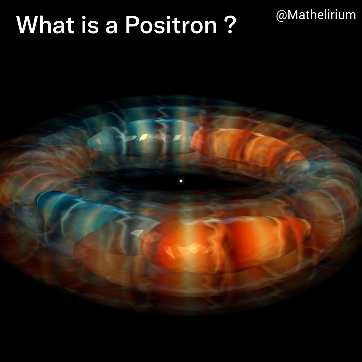


![Quantum Mechanics Series Lecture 4 Lecture 1 established that ρ(x,t) = |ψ(x,t)|² behaves like a conserved probability density. Lecture 2 showed what drives that flow. We also saw that writing ψ = r exp(iθ) makes the probability current proportional to the phase gradient, making it clear that phase geometry literally steers the motion. Lecture 3 then showed that the centroid of that flow can move almost classically when the packet is tight and the external potential is smooth. However, that raises yet another question. If the centroid can look classical, why does the full wave still spread, bend, split, and interfere in ways no classical particle cloud would? This is because the wave is not driven only by the external potential. It is also driven by its own curvature. Write ψ(x,t) = r(x,t) exp(iθ(x,t)) with ρ = r². Then Schrödinger’s equation gives two coupled real equations. One is the continuity equation you already know. The other looks like a Hamilton-Jacobi equation, but with one extra term: Q = −(1/2m) ∇²r / r This is the so-called Quantum Potential. It depends entirely on how the amplitude bends across space. So, the wave is being shaped not only by V(x,t), but also by the geometry of its own envelope. In the animation, the upper surface is still |ψ| and its skin is still colored by arg(ψ). The glowing threads still trace the probability current. But now a second membrane hangs underneath. That lower membrane encodes the quantum potential Q itself. The porcelain bead marks the quantum centroid. The amber bead follows a classical centroid under the same external V. When those paths separate, the lower membrane tells you why. The difference is not magic but the extra term classical mechanics does not have. The math breakdown: Start from Schrödinger evolution in units with ħ = 1: i ∂ψ/∂t = [ −(1/2m) ∇² + V(x,t) ] ψ Write the state in polar form: ψ = r exp(iθ) Then ρ = |ψ|² = r² From the imaginary part, you recover probability conservation: ∂ρ/∂t + ∇·j = 0 with j = (1/m) Im(ψ* ∇ψ) = (ρ/m) ∇θ So the local velocity field is v = j / ρ = ∇θ / m Now take the real part of Schrödinger’s equation. That gives ∂θ/∂t + |∇θ|² / (2m) + V + Q = 0 where Q = −(1/2m) ∇²r / r This is the classical Hamilton-Jacobi equation with one extra term. That extra term is what makes quantum motion locally different from classical motion. Take a gradient of that phase equation and use v = ∇θ / m. Then the flow obeys an Euler-like equation: ∂v/∂t + (v·∇)v = −(1/m) ∇(V + Q) In other words, there are really two forces in the problem. One comes from the external potential V. The other comes from the wave’s own curvature through Q. That is why Ehrenfest is only approximate. The centroid can still satisfy d⟨x⟩/dt = ⟨p⟩/m d⟨p⟩/dt = −⟨∇V⟩ but the internal shape of the packet evolves under the combined influence of V and Q. When the packet stays broad and smooth, Q is gentle and the motion looks more classical. When the packet develops sharp curvature or interference structure, Q becomes strong and the classical picture breaks down. That is what this scene is designed to show live. #QuantumMechanics #Wavefunction #SchrodingerEquation #BornRule #ProbabilityCurrent #ContinuityEquation #Phase #EhrenfestTheorem #QuantumPotential #Madelung #HamiltonJacobi #MathematicalPhysics #Mathematics #Physics](https://image.24vids.com/tw-2044118124148973661/amplify_video_thumb/2044117901251072000/img/IXBMEKzfYfpY_xGi.jpg)


![String Theory Lecture 1 A String Does Not Move Like a Point A point particle traces a line through spacetime. A string traces a surface. This is the first geometric shift in String Theory. Particle mechanics asks where one object is at time t, so its history is a curve. String Theory asks where every point of an extended object is at worldsheet time τ, so we need another coordinate telling us where we are along the string. For a point particle x(t) So, for one input of time we get a position in Spacetime. For a string Xᵘ(τ,σ) Here τ plays the role of time on the worldsheet, while σ labels position along the string. Freeze τ and vary σ, and you see the string at one instant. Let τ move, and that curve sweeps out a two-dimensional surface... the worldsheet. The same comparison appears in the action. For a relativistic point particle, the geometric action measures worldline length S = −m ∫ ds If we parameterize the path by t, the action has one integral, one parameter, and one tangent vector dxᵘ/dt For a string, the same idea grows by one dimension. The action measures area, not length. In Nambu-Goto form, S = −T ∫ dτ dσ √[−det hₐᵦ] Here T is the string tension. It plays a role similar to mass, but for an extended object. It weights the area of a surface rather than the length of a line. The particle action has ∫ dt because the history is one-dimensional. The string action has ∫ dτ dσ because the history is two-dimensional. We are no longer summing along a path, we are summing over a surface. The geometry changes for the same reason. For the particle, one derivative is enough dxᵘ/dt For the string, the geometry is built from two derivatives: ∂τXᵘ and ∂σXᵘ The first tells you how the string changes as worldsheet time flows. The second tells you how the embedding changes as you move along the string. Together they define the induced worldsheet metric hₐᵦ = ∂ₐXᵘ ∂ᵦXᵤ In plain terms, hₐᵦ measures tangent lengths and tangent angles on the worldsheet. From it, the area element is dA = dτ dσ √[−det hₐᵦ] This, the Nambu-Goto action is the direct analogue of the point-particle length action. The point particle extremizes length and the string extremizes area. For calculations, people usually switch to the Polyakov action: S = −(T/2) ∫ dτ dσ √[−γ] γᵃᵇ ∂ₐXᵘ ∂ᵦXᵤ This describes the same classical string dynamics, but the algebra is cleaner. After choosing conformal gauge, varying with respect to Xᵘ gives (∂²/∂τ² − ∂²/∂σ²) Xᵘ = 0 This is the first real dynamical payoff... a two-dimensional wave equation on the worldsheet. For a point particle, the equation of motion tells you how one position evolves along one path. For a string, it tells you how an entire curve evolves, with waves traveling along it. The term ∂²Xᵘ/∂τ² measures acceleration in worldsheet time, while ∂²Xᵘ/∂σ² measures curvature along the string. The time evolution is balanced by how the string bends along its own length. This is why strings have oscillation modes. A point particle has one trajectory. A string has many possible vibration patterns, each one a normal mode of the worldsheet wave equation. For a closed string, σ wraps around the loop Xᵘ(τ, σ + 2π) = Xᵘ(τ, σ) For an open string, one standard free-end condition is ∂σXᵘ = 0 at the endpoints. Solving the wave equation gives waves moving in opposite directions along the string Xᵘ(τ,σ) = Fᵘ(τ + σ) + Gᵘ(τ − σ) A function of τ + σ moves one way. A function of τ − σ moves the other. Therefore, a particle has a worldline, its action measures length, and its geometry uses one tangent. The string has a worldsheet, its action measures area, and its geometry uses two tangent directions. #StringTheory #TheoreticalPhysics #MathematicalPhysics #Physics #Spacetime](https://image.24vids.com/tw-2047925796963004514/amplify_video_thumb/2047925638485753856/img/d0IV19m4OAIfEf0I.jpg)
